
Abstract
Aiming at the problems of low data reconstruction accuracy in wireless sensor networks and users unable to receive accurate original signals, improvements are made on the basis of the stagewise orthogonal matching pursuit algorithm, combined with sparseness adaptation and the pre-selection strategy, which proposes a sparsity adaptive pre-selected stagewise orthogonal matching pursuit algorithm. In the framework of the stagewise orthogonal matching pursuit algorithm, the algorithm in this article uses a combination of a fixed-value strategy and a threshold strategy to screen the candidate atom sets in two rounds to improve the accuracy of atom selection, and then according to the sparsity adaptive principle, the sparse approximation and accurate signal reconstruction are realized by the variable step size method. The simulation results show that the algorithm proposed in this article is compared with the orthogonal matching pursuit algorithm, regularized orthogonal matching pursuit algorithm, and stagewise orthogonal matching pursuit algorithm. When the sparsity is 35 < K < 45, regardless of the size of the perception matrix and the length of the signal, M = 128, N = 256 or M = 128, N = 512 are improved, and the reconstruction time is when the sparsity is 10, the fastest time between 25 and 25, that is, less than 4.5 s. It can be seen that the sparsity adaptive pre-selected stagewise orthogonal matching pursuit algorithm has better adaptive characteristics to the sparsity of the signal, which is beneficial for users to receive more accurate original signals.
Keywords
Introduction
Data compression performed by sensor nodes in wireless sensor networks (WSNs) before data transmission can effectively save energy and extend battery life. 1 In recent years, a large number of compression algorithms have been proposed and applied. They also have achieved remarkable results. After the signal is sent out, the space occupied by the signal is reduced by compression, and the original signal is restored through signal reconstruction after reaching the destination node.
In terms of signal reconstruction, the main algorithms include the minimum convex optimization algorithm, combination algorithm, and greedy algorithm.
2
The main idea of the
The greedy algorithm is the earliest proposed matching pursuit (MP) algorithm. 6 The atom selection strategy of the MP algorithm is to select the atom with the highest degree of matching with the residual from the observation matrix as the candidate atom. This atom selection strategy can be guaranteed to become high accuracy, but the orthogonality between the iterative residual and the selected atom set cannot be guaranteed. This makes the approximate solution obtained by MP suboptimal in the sense of the optimal K term approximation. The orthogonal matching pursuit (OMP) algorithm 7 improves the MP algorithm. The OMP algorithm uses the least squares method to update the linear combination coefficients of the selected atoms each time the set of selected atoms is updated. However, the MP and OMP algorithms are not ideal in reconstruction efficiency and accuracy. 8 Needell D and Vershynin R. proposed a regularized orthogonal matching pursuit (ROMP) algorithm on the basis of the OMP algorithm, 9 using the regularization method which finds the atom set with the largest energy in the candidate atom set to update the support set. Donoho D and Tanner J. proposed a stagewise orthogonal matching pursuit (StOMP) algorithm. 10 By setting a threshold, atoms are selected in batches instead of simply selecting the atom with the highest degree of matching with the signal. This can improve the efficiency of the algorithm, but the reconstruction accuracy is poor. At the same time, the above greedy algorithms all require that the sparsity of the signal is known. If the sparsity estimation is not accurate, many signals will not be accurately reconstructed, but this premise is difficult to meet in practical applications. 11 Thong T et al. proposed the sparsity adaptive matching pursuit (SAMP) algorithm. 12 This algorithm is not affected by signal sparsity. It is used in preseting the initial step size and adding a fixed value in each iteration. The step size gradually realizes the estimation of the signal sparsity, and at the same time updates the residual and the support set to approximate the original signal, but overall, the reconstruction efficiency of the algorithm is low. 13
Aiming at the problem of low reconstruction rate, this article proposes a pre-selection strategy to enhance the accuracy of the algorithm in the atom selection stage. The atom selection part is refined, it is carried out in two steps. First, the atoms are selected through a fixed-value strategy, the atoms after the primary selection are used as candidate atoms in the reselection stage. In the reselection stage, a threshold selection strategy is used to screen the candidate atoms a second time. After the reselection stage is completed, the atoms that pass the screening twice will be added to the support set to participate in the signal reconstruction. Finally, according to the principle of sparsity adaptation, the step size is used to achieve the staged selection of atoms in the candidate set. As the iterative process is carried out in segments, the step size and support set are continuously updated. And finally, the third screening of atoms is achieved. This approach enables the reconstructed signal to recover the original signal more accurately, and the reconstruction efficiency of the algorithm is also improved. Compared with the traditional algorithm, the atom is screened three times, so that the screened signal is closer to the original signal. After reconstruction, the original signal is recovered more accurately and the reconstruction efficiency of the algorithm is improved, the node storage cost and communication overhead are reduced, and the sampling efficiency is indirectly improved, which lays a solid foundation for the subsequent data transmission of the WSN.
Basic theory of compressed sensing
Compressed sensing includes three contents, which are the sparse representation of the signal, the measurement of the observation matrix, and the reconstruction algorithm. In the mathematical model of compressed sensing: 14

where x represents the original signal, A represents the sparse mapping matrix, and y represents the compressed measurement. The process of sparse representation is that the original signal can be reflected into a small vector space through the sparse mapping matrix A, and the number of rows in the vector space after the effect will be much less. This process is actually the core idea of sparse theory, which is to use low-dimensional signals to describe high-dimensional signals. 15 The specific compression process is as follows: first, sparsely represent the signal on an orthogonal basis Ψ, then determine an observation basis Φ, which needs to be uncorrelated with Ψ, then the observation value Y can be obtained by y = Φx, and finally, Y is optimized and reconstructed. The mathematical model of compressed sensing is shown in Figure 1.

Mathematical model of compressed sensing.
Sparse representation of the signal
If the signal x ∈ RN of length N has only K coefficients that are not 0 (or obviously larger than other coefficients) in a certain transform domain, and K << N, then the signal x is sparse in this transform domain, also called K-sparse.
16
If the signal on the sparse basis matrix

Observation matrix measurement
Obtain M(K << M << N) linear projections on the measurement basis

Compressed sensing algorithm reconstruction
Starting from the M measured values, the original signal x is reconstructed or approximated with the help of the observation matrix Φ and the reconstruction algorithm. In the case where x is K-sparse, the reconstruction of the signal can be equivalent to the problem of the optimal solution under the constraints, 18 which is expressed as follows:


Feasibility analysis based on threshold reconstruction
The sparsity adaptive pre-selected segmented OMP algorithm proposed in this article uses threshold indicators to select atoms when the signal sparsity is unknown. In this section, we will use the constraint isometric property to prove that the sparsity of the algorithm is unknown, but the threshold can still accurately reconstruct the original signal. The definition of constrained isometric properties is presented below.
Definition 3.1 19
For any K-sparse signal x and the constant δK∈(0,1), if

then it is said that matrix A satisfies the K-order constrained equidistant property, and δK is called the K-order constrained equidistant constant, where the index I∈{1,2,…, N} and |I|≤ K, AI is only corresponding to matrix A for the sub-matrix composed of the columns of the index set I, and |I| represents the number of elements contained in the index set I.
Lemma 3.1 19
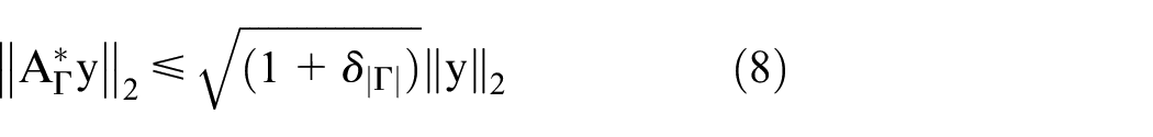
If matrix A satisfies the s-order constraint equidistance, then for any index that satisfies the condition s ≥|Γ| Set Γ and any x∈RN, y∈R|Γ,| the following formula holds:

Lemma 3.2 19
Assuming that Γ and Λ are two disjoint sets, if A satisfies the |Γ∪Λ| order constraint equidistance with constant δ|Γ∪Λ,| then for any x∈R|Λ| has the following formula:

Lemma 3.3 19
For any two integers K1 and K2 satisfying the condition K1 ≤ K2, there are

Established
Let C be the support set of the signal obtained at the termination of the algorithm proposed in this section and satisfy q = |C.| The following proves that the algorithm estimates the signal xj (1, 2,…, L) feasibility.
Corollary 2.3.1
Denote the index set Λ ={I1, I2,…, Is}, let s∈N and s ≤ q, matrix A satisfies the q+s-order constraint equidistance with constant δq+s and
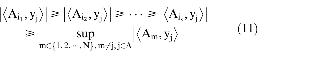
then there is

yes, where yj =Axj = ACxj(C).
Proof
Use the method of proof by contradiction. Suppose Λ∩ C ≠∅, then from equation (9):

Note that

where|xj| is the vector composed of the absolute values of the components of vector xj. Obviously
Among them, C\
However, according to formula (9), we have
So there is

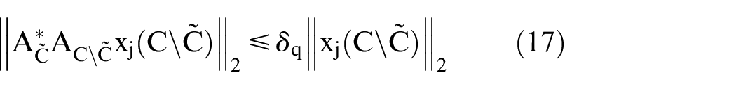
According to formulas (13) and (18), there are

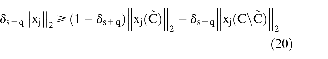
From equations (10) and (19), there are
If the elements of |xj| are arranged in descending order, that is
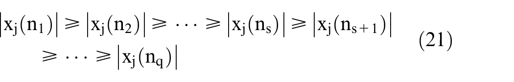
Then
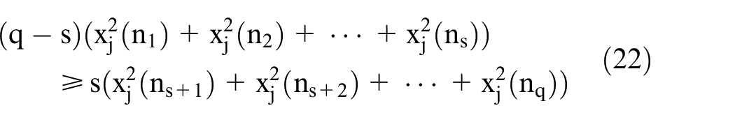
In fact, there are s(q – s) terms on both sides of equation (22) but the terms on the left are greater than or equal to the terms on the right. Based on formula (22), we have

From the definition of the index set

Noticed
Then

Because of equation (20), equations (24) and (26) have
In other words

considering

then
which is

Obviously, formula (31) is contradictory to the assumption of Corollary 3.1. Therefore, Λ∩ C ≠∅. The certificate is complete.
Corollary 3.1
This shows that although there is no signal sparsity as a priori information, the threshold mechanism proposed in this article can still ensure that at least one correct index for the signal xj can be found by the algorithm in the first iteration, which is an accurate reconstruction of the original signals that lay the foundation.
Segment OMP algorithm improvement
Piecewise OMP algorithm
The StOMP algorithm is a greedy algorithm improved from the OMP algorithm. 20 The greedy algorithm selects the 2K or K atoms, whose inner product is the largest in the iterative process. The StOMP algorithm determines the atoms through a threshold, and the input parameters do not include the signal sparsity K. Compared with the ROMP algorithm, the StOMP algorithm has higher computational efficiency and reconstructed signal accuracy. 21 However, the StOMP algorithm still has a problem, which is the setting of the threshold. The threshold cannot be too large or too small. If the value is too large, the calculation efficiency will be reduced; if the value is too small, it will increase the possibility of wrong atom selection. Although a threshold selection range is given as 2≤α≤3, because the selection of the threshold has a great influence on the effect of the algorithm, this range still appears to be very broad and needs to be precise again. 22 In order to reduce the low signal reconstruction efficiency caused by improper selection of the threshold, this article proposes a combination of pre-selection strategy and adaptive sparsity, which is used to enhance the accuracy of the algorithm in the atomic selection phase. Thus, while improving the reconstruction efficiency, the accuracy of signal reconstruction is ensured. In this article, the SAPStOMP algorithm, StOMP algorithm, OMP algorithm, and ROMP algorithm are further simulated. The comparison between several algorithms verifies that the SAPStOMP algorithm has obvious advantages compared with other algorithms.
Principles of algorithm improvement
Greedy algorithms generally use an atomic selection strategy to complete the selection of atoms, in which the atom screening part will indirectly affect the signal reconstruction efficiency. In this article, the atom screening part is refined and the atom is screened in two rounds using the pre-selection strategy. The pre-selection strategy will use a combination of two strategies, namely, a fixed-value selection strategy and a threshold selection strategy. Among them, the fixed-value strategy is a simple improvement strategy to the serial atom selection strategy. Different from the serial atom selection strategy, only the atom with the largest inner product of the residual is selected to be added to the support set. The fixed-value selection strategy selects L matching atoms in each iteration, where L is less than sparsity K; the threshold strategy is to judge whether the candidate atoms meet a predetermined threshold condition. Since the number of atoms meeting the threshold condition in each iteration is uncertain, the number of atoms selected in each iteration is also uncertain. These atoms that meet the threshold conditions will be put into the support set and participate in the subsequent signal reconstruction.
The algorithm in this article performs the third screening in the support set. The sparsity adaptive process is used this time. This process is to find a suitable estimated sparsity to approximate the true sparsity of the signal. If this article defines an ideal support set ΛT as a support set that contains all the correct atoms and only the correct atoms, the sparsity K of the signal is actually the potential of the ideal support set, namely, |ΛT| = K. When the signal sparsity K is unknown, the sparsity adaptive sets the initial step size to form an atom candidate set, determines the number of atoms in the candidate set and the current step size, and completes the support set update according to the judgment result. The long update completes the approximate estimation of the sparsity and makes the signal reconstruction more accurate.
In the pre-selection strategy section, there will be two choices of atomic pre-selection and atomic reselection. If the atomic selection is regarded as the interview of the reconstruction algorithm on the atoms in the observation matrix, then the atomic pre-selection and the atomic reselection are similar to the initial and retests in the interview. First, the primary selection of atoms is performed through a fixed-value strategy, and then the primary selected atoms are regarded as candidate atoms in the reselection stage. In the multi-selection stage, the threshold selection strategy is adopted. The atoms selected in the multiple selection phase will be screened for the third time. The third screening process is related to the step length. When the number of candidate sets is small, the next iteration takes a large step. The support set can be effectively expanded to achieve the goal of approaching sparsity. When the number of candidate sets is large, in order to prevent the overestimation of sparsity, this article adopts a small step size to filter atoms and approximate sparsity. By changing the step size by identifying the parameters, the support set can be expanded more effectively and the sparsity of self-adaptive estimation can be achieved, so as to achieve the purpose of improving signal reconstruction performance.
The SAPStOMP algorithm uses the pre-selection strategy as the atomic selection strategy, and effectively expands the support set in combination with sparsity adaptation. It is worth noting that the number of atoms selected in each iteration as the threshold strategy of the primary selection is not fixed. Therefore, it is possible that the number of atoms passing the pre-selection is less than the number of atoms to be “admitted” for the double selection. In this case, the SAPStOMP algorithm treats all atoms that have passed the primary selection as automatic check-selection, and put them directly into the support set. The sparseness adaptive part after that is equal to the third selection, which improves the accuracy of reconstruction. The algorithm flow of the sparsity adaptive pre-selected segmented OMP algorithm is shown in Figure 2.
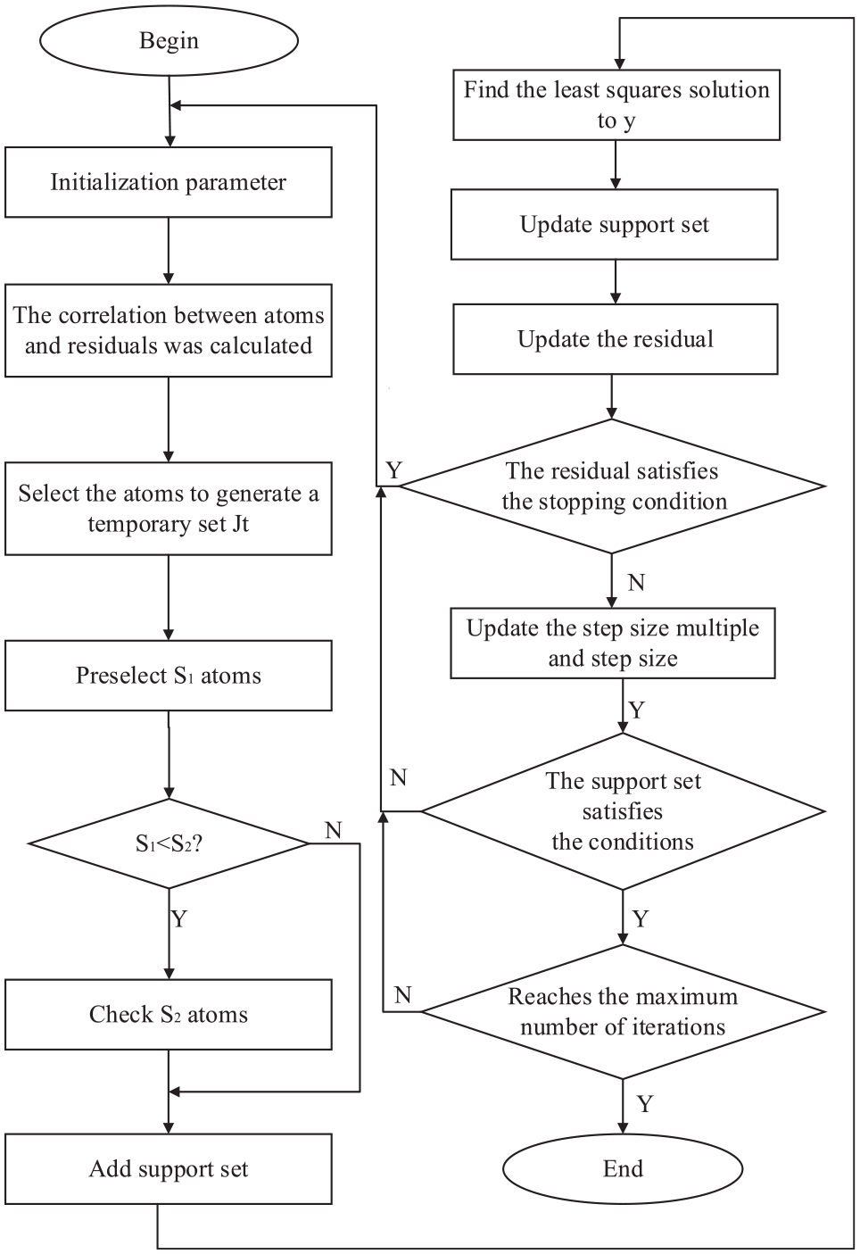
Sparsity adaptive pre-selected segmented orthogonal matching pursuit algorithm flow.
Improved algorithm steps
The symbol description is as follows: y is the observed vector, the size is M×1, y = Φx; x is the original signal, which is generally not sparse, but in a certain transform domain Ψ is sparse, and the size is N×1 (M << N); θ is K-sparse, which is the sparse representation of the signal in x in a certain transform domain; Φ is the measurement matrix, the size is M×N; Ψ is the sparse matrix, the size is N×N; A is the sensing matrix, the size is M×N, generally K << M << N. The sparse representation model in compressed sensing is x = Ψθ, so the sensing matrix A = ΦΨ.
In the following process, rt represents the residual, t represents the number of iterations, Ø represents the empty set, Λt represents the index (column number) set of t iterations (the number of elements is L, L is equal to the integer multiple of the step size ST), aj represents the jth column of matrix A, A ={aj}(for all j∈CK) represents the column set of matrix A selected by index set CK (let the number of columns be Lt), θt is the column vector of Lt×1, the symbol ∪ represents the set union operation, <·,·> represents the inner product of vectors, and abs[.] represents the modulus value (absolute value).
Input: M×N sensing matrix A = ΦΨ; N×1 dimensional observation vector y; total number of iterations S, default is 10; threshold parameter α, default is 2.5; step size ST; step size multiple stage. Output: signal sparse representation coefficient estimation
Step 1. Initialization: r0 = y, Λ0 =∅, A0 =∅, Lt = ST, t = 1, Stage = 1.
Step 2. Calculate the correlation degree:
Step 3. Primary selection: select the maximum value of Lt in ut, and form a set Jt (column sequence number set) corresponding to the column number j of A to generate a temporary set Jt.
Step 4. Check:
1. If Jt ≥ Lt, generate set
2. If Jt < Lt, add all the atomic indexes that passed the primary selection to the support set that
3. If no new column is selected that
Step 5. Find the least squares solution of
Step 6. Generate a new support set: select the Lt item with the largest absolute value from
Step 7. Update the support set:
Step 8. Update the residual:
Step 9. Determine the stop condition:
1. If rt = 0, stop the iteration and proceed to step 11; if
2. If ΛtL ≥ L, stop the iteration and go to step 11, otherwise go to step 10;
3. If t = S, stop the iteration and proceed to step 11, otherwise return to step 2 to continue the iteration.
Step 10. Update the number of iterations: t=t+1.
Step 11. The reconstructed
Note 1. After obtaining
Note 2. It can be known from the input parameters that this algorithm does not need to know the signal sparsity K;
Note 3. When the measurement matrix is a random Gaussian matrix, the threshold Tn = ασt, where the value range of α is generally 2 ≤ α ≤ 3, and the noise level σt = ||rt||2/
Note 4. The variance is 1/M, in other words, the standard deviation is 1/
Step 1 of the algorithm is initialized, where the initial step size ST cannot be too large or too small. Too large will reduce the reconstruction quality, and too small will increase the reconstruction time. In practice, it is necessary to select a suitable value according to different goals. In order to obtain a higher reconstruction quality, this article chooses s = 1; step 2 selects the atom closest to the residual through the inner product of the atom and the residual; step 3 uses a fixed-value strategy to perform the primary selection of the atom, and selects L matches in each iteration step 4, check the atoms, get the atom candidate set Jt of the current iteration by setting the threshold αt, then put it into the support set, and use the support set Λt for signal estimation; step 5 Find the least squares solution, and use the orthogonalization idea to calculate the reconstructed signal to make the result more accurate; step 6 uses the least square method to obtain a more effective support set F, and through the third selection of atoms in the candidate set, some irrelevant atoms are removed, and finally formed really support set to achieve better reconstruction performance; step 7 calculate the residual r based on the support set of step 6; step 8 determine whether the stopping condition is satisfied. If satisfied, the output signal is sparse and express the coefficient estimate
Experimental simulation
In order to verify the effectiveness of the pre-selected segmented OMP algorithm, a simulation experiment was carried out on the improved algorithm. Because the Gaussian matrix can satisfy the constraint equidistance with extremely high probability, the randomly generated Gaussian sparse signal x∈RN and the Gaussian matrix Φ∈RM×N with variable sparsity K are used as the original signal and for the observation matrix, the value range of K is [1, 80]. When the observation matrix is a Gaussian random matrix, the threshold parameter of StOMP and the algorithm in this article is set to 2.5.
The simulation experiment was carried out with MATLAB 7.0 software under Microsoft 64-bit Win 10 system, and it took 4937.843,156 s to run. In the simulation experiment, the probability and time of accurate signal reconstruction by each algorithm are the main evaluation criteria. The unit of time is second (s), and the probability of accurate signal reconstruction is expressed in percentage (%). In the simulation experiment, each experiment is conducted for 1000 times, and the average probability and time of accurate signal reconstruction of 1000 times of experiment are taken as the final probability and time of accurate signal reconstruction.
In this experiment, compare the correct reconstruction probability and reconstruction time of OMP, ROMP, StOMP, and SAPStOMP algorithms under different sparsity conditions. In order to compare the reconstruction effects of various algorithms under different sparsity, the size of the perception matrix and the length of the signal are respectively taken as M = 128, N = 256 and M = 128, N = 512.
The size of the perception matrix and the length of the signal taken in Figure 3 are M = 128 and N = 256, respectively. It can be seen from the figure that ROMP is suitable for a lower sparsity environment; when K = 40, the OMP algorithm’s reconstruction performance is significantly lower than that of the StOMP algorithm and the SAPStOMP algorithm; for the signal with sparsity K = 45, the improved algorithm, StOMP algorithm, OMP algorithm, and ROMP algorithm have respectively 98.89%, 49.82%, 24.11%, and 24.11%. The SAPStOMP algorithm can accurately recover the original signal for all signals with a sparsity less than 45. In a higher sparsity environment, the SAPStOMP algorithm also has an advantage over other algorithms in terms of reconstruction accuracy. In general, the SAPStOMP algorithm has the best reconstruction performance under different sparsity.

Reconstruction performance of each algorithm under different sparsity (N = 256).
The size of the perception matrix and the length of the signal taken in Figure 4 are M = 128 and N = 512. Compared with Figure 3, the signal length is changed and the simulation is performed again. It can be seen that the ROMP algorithm has a signal length of N = 512. In this case, it is also applicable to environments with lower sparsity; under the same sparsity K, the probability of accurate signal reconstruction of the SAPStOMP algorithm is higher than the other algorithms in all algorithms. For the convenience of comparison, the probability of accurate reconstruction of each algorithm is compared with K = 40 as an example. At this time, the accurate reconstruction probability of each algorithm is 60.81% of SAPStOMP algorithm, 51.64% of StOMP algorithm, SAPStOMP algorithm is 9.17% better than StOMP algorithm, 26.14% of OMP algorithm, and 0% of ROMP algorithm from high to low. When the sparsity is 35 < K < 45, the SAPStOMP algorithm has advantages over other algorithms, but in other sparsity situations, the effect of the SAPStOMP and StOMP algorithms is not much different, and both are in the first echelon, which is better than other algorithms. In general, the SAPStOMP algorithm is more suitable for the 35 < K < 45 environment when the signal length is 512, and it still needs to be improved in other sparsity environments.

Reconstruction performance of each algorithm under different sparsity (N = 512).
Through the above two groups of simulation experiments, it can be seen that for short signals (N = 256), the SAPStOMP algorithm has a better probability of accurate signal reconstruction than other algorithms. For signals with long length (N = 512), under the same sparsity K, the SAPStOMP and StOMP algorithms have little difference in probability of accurate signal reconstruction. Therefore, when the sparsity is 10 to 25, the reconstruction time of each algorithm is compared and analyzed.
Figure 5 compares the reconstruction time of each algorithm under different sparsity, and finds that the SAPStOMP algorithm takes the shortest reconstruction time under the same sparsity. For example, when K = 20, the OMP algorithm takes the longest time and the SAPStOMP algorithm takes the shortest time; when K = 25, the SAMP algorithm takes longer to reconstruct than the OMP algorithm. The improved algorithm in this article still takes longer and is the shortest. The lesser the time required for reconstruction, the faster the user can obtain the original signal.

Reconstruction time of each algorithm under different sparsity.
It can be seen from the above simulation results that the SAPStOMP algorithm is significantly better than the OMP algorithm, ROMP algorithm, and StOMP algorithm in terms of the accuracy of the reconstructed signal and the signal reconstruction time.
Conclusion
In view of the short reconstruction time of the StOMP algorithm but low reconstruction accuracy, this article improves on the original StOMP algorithm and proposes the SAPStOMP algorithm. The SAPStOMP algorithm uses the combination of a threshold strategy and a fixed-value strategy to improve the accuracy of atomic screening, and uses step conversion to improve the reconstruction efficiency. The initial stage uses a large step to increase the reconstruction speed, and the subsequent stage uses a small step and long approximation to the true sparsity of the signal, and finally realizes the accurate reconstruction of the signal. At the same time, a simulation comparison experiment was carried out to compare the reconstruction efficiency and the time of the improved algorithm, OMP algorithm, ROMP algorithm, and StOMP algorithm. Experiments show that the SAPStOMP algorithm has higher reconstruction efficiency and shorter reconstruction time than the OMP algorithm, ROMP algorithm, and StOMP algorithm. Therefore, the algorithm in this article not only has high reconstruction quality, but also has certain advantages in reconstruction time. It is a better reconstruction algorithm. But there are still shortcomings in this article: the proposed algorithm needs further improvement; this article applies it directly to the default parameters in atom selection phase 2.5; this can be a further refined study with more appropriate threshold parameters; the algorithm has a signal length of 512 cases, only in the sparse degree of 35 < K < 45, whereas in other parts, the sparse degree of refactoring rate still needs to be improved.
Footnotes
Handling Editor: Peio Lopez Iturri
Declaration of conflicting interests
The author(s) declared no potential conflicts of interest with respect to the research, authorship, and/or publication of this article.
Funding
The author(s) disclosed receipt of the following financial support for the research, authorship, and/or publication of this article: The authors wish to thank the Scientific Research Project of Science and Engineering Talents Program of Harbin University of Science and Technology (No. LGYC2018JC047) and Heilongjiang Provincial Leading Talent Echelon Reserve Leader Funding for their support.