Sage Journals: Discover world-class research

Abstract

Autism is a neurodevelopmental disorder that cannot be completely cured, but early intervention during childhood can improve outcomes. Identifying autism spectrum disorder (ASD) has relied on subjective detection methods that involve questionnaires, medical professionals, and therapists and are subject to observer variability. The need for early diagnosis and the limitations of subjective detection methods has led researchers to explore machine learning-based approaches, such as Random Forests, K-Nearest Neighbors, Naive Bayes, and Support Vector Machines, to predict ASD meltdowns. In recent years, deep learning techniques have gained traction for early ASD detection. This study evaluates the performance of various deep learning networks, including AlexNet, VGG16, and ResNet50, using 5 cepstral coefficient features for ASD detection. The main contributions of this study are the utilization of Cepstral Coefficients in the processing stage to construct spectrograms and the modification of the AlexNet architecture for precise classification. Experimental observations indicate that the AlexNet with Linear Frequency Cepstral Coefficients (LFCC) yields the highest accuracy of 85.1%, while a customized AlexNet with LFCC achieves 90% accuracy.

Keywords

autism cepstral coefficients AlexNet VGG16 ResNet50

Introduction

Autism spectrum disorder (ASD) is a complex disorder characterized by communication and behavioral issues. Autism can be identified if an individual faces continual difficulty with social communication, restricted interests, and repetitive behavior.1 The condition can be identified as early as at the age of 16 months, but it remains difficult due to the absence of any physical traits in autistic children. In a typical method, doctors will utilize an early childhood screening tool to detect autism in children aged 16 to 30 months. However, doctors’ lack of expertise and training can and have resulted in incorrect diagnoses.² The observed increase in ASD prevalence estimates is expected to have a serious impact on the living conditions of families that care for children with ASD. According to studies, the lifetime economic cost of ASD might reach up to $2.4 million per afflicted individual.³ Therefore, it is particularly important to advance research on ASD across all populations and geographies, especially in countries like India that have low-middle income (LMICs).⁴ The Autism Diagnostic Observation Schedule is widely regarded as the universal standard for autism assessment.⁵ The Autistic Diagnostic Interview-Revised (ADI-R)and DSM-5 to gather data to observe the pattern of autism symptoms throughout adolescence and adulthood.^6,7 Parent training, Cognitive-Behavioral Therapy (CBT), Treatment and Education of Autistic and Related Communication-Handicapped Children (TEACCH), and applied behavioral analysis are all treatment options for autism.⁸ Due to the delayed response of the brain's circulatory system as well as fMRI imaging time limits, fMRIs have poor temporal resolution even though they have high spatial resolution and are not optimal for recording the quick changes of brain activity. Furthermore, these approaches are highly sensitive to motion artifacts.⁹ The diagnosis of ASD can be aided by a combination of psychophysiological data, which may include EEG, fMRI, eye movement data, and thermal images.^10,11

The most extensively utilized method for detecting brain activity is electroencephalography (EEG).¹² The EEG signal has a high resolution in time (milliseconds), and it allows for accurate temporal assessment of brain activity. The overwhelming majority of the evidence points to severe connection abnormalities in ASD that may be pervasive and have 2 distinct aspects: under-connectivity in long-distance networks and over-connectivity in local networks. Additionally, it was noted that disturbances seem to worsen in later-developing brain regions like the prefrontal cortex. Based on the findings from the reviews related to EEG, it is plausible that increased brain excitability may be a factor in the important overlap between ASD and epilepsy, possibly contributing to the connection. Focused observations taken across multiple settings (such as home and nursery) are included in observational assessments. There has been substantial development in machine learning (ML) algorithms and deep learning (DL) for autism diagnosis in recent years.^13,14 This research attempts to demonstrate a novel method for autism detection, by using Cepstral Coefficients to generate spectrograms of EEG signals. Then, using a customized version of AlexNet, the spectrograms were classified as ASD or Typically Developing (TD).

Related Works

Haputhanthri et al proposed a method to extract statistical features from EEG data after Discrete Wavelet Transform and utilized correlation-based feature selection to choose relevant features and EEG channels. They reported better accuracy by employing random forest with selected features, such as means of FT9, P3, and Oz channels, and standard deviations of TP9 and FC2 channels.¹⁵ Moreover, Haputhanthri et al performed a study to extract mean, standard deviation, and entropy values of EEG signals and mean temperature values of regions of interest in facial thermographic images as features. They used correlation-based feature selection to filter out less informative features. The classification process was carried out using Naive Bayes, random forest, logistic regression, and multilayer perceptron algorithms. The integration of EEG and thermographic features resulted in better accuracy with both logistic regression and multilayer perceptron classifiers.¹⁶

Mohanta et al conducted a test where speech signal datasets were recorded in English, of children with ASD and TD who were non-native Indo-English speakers, and their following acoustic features were obtained and it used for classify activities of ASD and normal children: fundamental frequency (FO), strength of excitation, formants frequencies (F1-F5), dominant frequencies (FD1, FD2), zero-crossing rate, signal energy (E), Mel-frequency cepstral coefficients (MFCC), and linear prediction cepstral coefficients. These feature sets were further classified using various classifiers, of which the classifier model based on K-Nearest Neighbors achieved better accuracy compared to other standard models.¹⁷ Cooney et al investigated the relative impacts of different attributes on classification accuracy by recording a dataset of imagined speech. These data were then used to generate 3 unique feature-sets: a linear feature-set, a nonlinear feature-set, and a feature-set consisting solely of MFCC. An support vector machine (SVM) classifier and a decision tree classifier were trained using each feature set, and the results showed that using MFCC features gives better differentiation of EEG recordings of imagined speech than the other features tested, and that phonetic distinctions between imagined words can help with classification.¹⁸

Tawhid et al proposed a method that involved preprocessing techniques, such as re-referencing, filtering, and normalization, to preprocess raw EEG data. The preprocessed EEG signals were transformed into 2-dimensional images using short-time Fourier transform (STFT), and textural features were extracted from these images. Principal component analysis (PCA) was then applied to select significant features, which were fed into an SVM classifier for classification.¹⁹ In another study by Tawhid et al, the preprocessed signals were transformed into 2-dimensional spectrogram images using STFT. The images underwent separate evaluations using ML and DL models. In the ML process, textural features were extracted, and PCA was applied to select significant features, which were fed to 6 distinct ML classifiers for classification. Meanwhile, in the DL process, 3 different convolutional neural network (CNN) models were evaluated.²⁰

Baygin et al utilized a one-dimensional local binary pattern (1D_LBP) to extract features from the EEG signal. The features were then used as input to generate spectrogram images through STFT. A hybrid deep lightweight feature generator, combining pretrained MobileNetV2, ShuffleNet, and SqueezeNet models, was utilized to extract deep features from the generated spectrogram images. A 2-layered ReliefF algorithm was employed for feature ranking and selection, and the most discriminative features were fed to an SVM classifier for automated autism detection.²¹ Hidir et al reviewed various studies that employ DL for the diagnosis of ASD based on structural and functional magnetic resonance imaging and a few hybrid imaging techniques, in the last 10 years. Their conclusion was that automated ASD detection employing DL approaches and brain sMRI and fMRI data has not yet attained the desired degree of success and cannot help in the early or speedy diagnosis of ASD.²² More image datasets with more images, more practical feature extraction techniques, and more dependable and versatile ML or DL models are required.

Furthermore, training a DL model with image data from different demographics will improve its reliability. Even though DL has been applied to solve a variety of neuroscience problems, their use in autism diagnosis has been minimal thus far. DL models such as CNN, which performs automatic feature extraction, and stacked autoencoder, which maintains a high feature level, have the potential to provide reliable ASD diagnosis. ML approaches have produced beneficial solutions, as illustrated by the works mentioned above. DL has a benefit over simple ML in that it can automatically engineer features, instead of manual extraction of features. Furthermore, when working with shapeless data, DL models provide significantly better performance metrics. Putting these advantages of DL to use, a novel system has been developed to classify ASD and TD with high accuracy in this paper.

Proposed System

Figure 1 demonstrates an overall view of the procedure for the proposed methodology for ASD detection.

Figure 1.

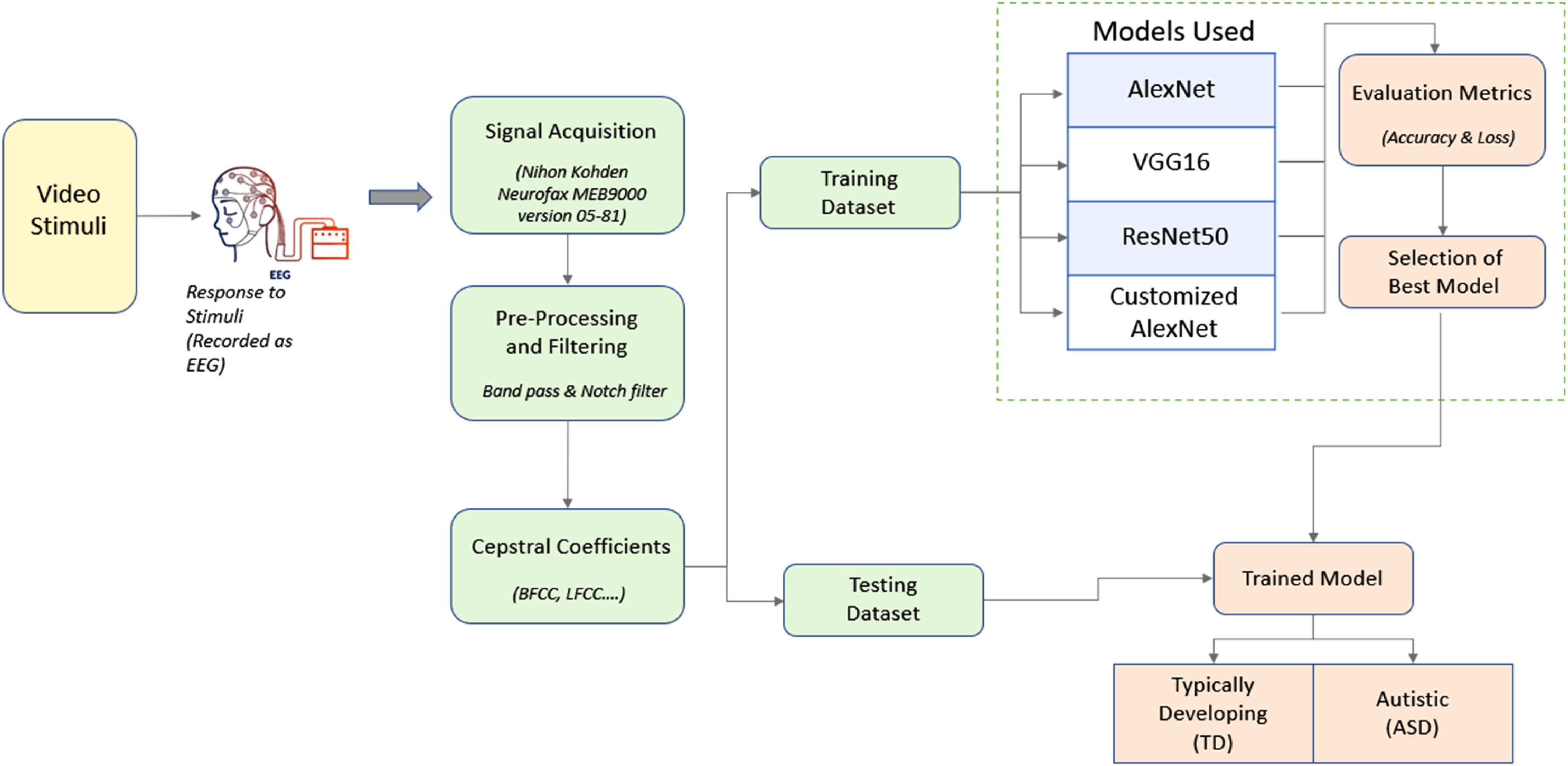
Block diagram of the proposed system.

Data Acquisition

Twenty children participated in the study in total, 10 of whom had ASD and 10 of whom had TD. DSM V was used to evaluate the cognition level of the participants beforehand. The children with ASD and TD who took part in the study ranged in age from 5 to 7 years. Prior to participation, the participants signed consent forms acknowledging that their EEG data would be reviewed and used for study purposes. The strategy for this research was following the “Helsinki Ethical Principles and ICMR Ethical Guidelines” handbook.²³ The participants were seated in a comfortable chair in a dark and silent area.

Stimuli selection

With practice, the children with autism became used to the electrode placements and were trained to sit and watch the videos without making any unexpected movements. The focus level of ASD children toward the offered stimuli could not be seen visually very clearly. The capture of EEG signals during the presentation of stimuli can offer a better understanding of their concentration level. As part of the stimuli creation process, every participant was instructed to watch 5 videos, with each video having duration of 2 min.

Preprocessing

Raw EEG data were filtered with a band-pass filter with a cutoff frequency of 0.53 to 70 Hz. A band-stop filter was employed to remove the overhead power line interference noise of 50 Hz so that it does not disrupt neural activity.

Feature Extraction

EEG signals contain information at different frequencies, which can be related to different brain activities. Cepstral analysis provides a way to separate the different frequency components of the EEG signal and extract features that capture this information. Cepstral coefficients as a feature extraction technique in EEG analysis because they provide an effective way to extract spectral characteristics from the complex EEG signal of audio-video stimuli. Five different cepstral coefficients’ spectrograms were extracted, namely, Bark Frequency Cepstral Coefficients (BFCC), Gammatone Frequency Cepstral Coefficients (GFCC), Linear Frequency Cepstral Coefficients (LFCC), MFCC, and Normalized Gammachirp Cepstral Coefficients (NGCC). Figure 2 shows the general process of extracting a cepstral coefficient from the EEG signal.

Figure 2.

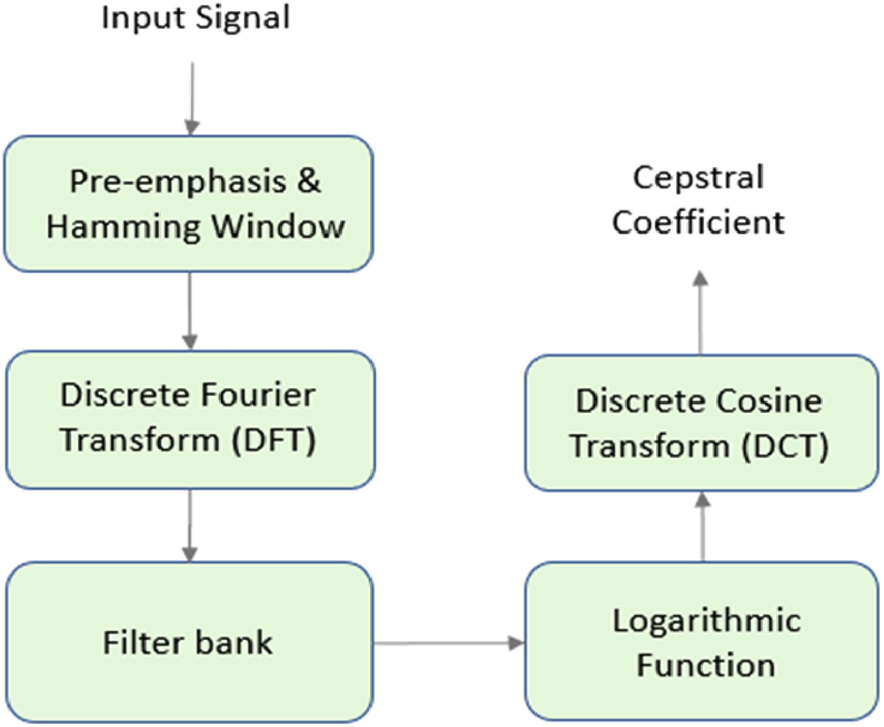
Generalized block diagram of the extraction process of a Cepstral coefficient.

The “Filter bank” in the above process is replaced by the Mel frequency scale, Bark frequency scale, Linear frequency scale, Gammatone filter bank, or a Normalized Gammachirp filter bank to extract their respective Cepstral Coefficients. MFCC use mel scale filter bank can improve the accuracy of EEG analysis by mimicking the nonlinear frequency sensitivity of the human auditory system. LFCC use linear scale filter bank can be useful in EEG analysis when precise frequency information across the entire spectrum is needed, such as in some types of event-related potential studies. BFCC use bark scale filter bank provides improved frequency resolution and reduced noise in analyzing EEG signals related to auditory processing. GFCC use gammatone filter bank can provide improved frequency selectivity in analyzing EEG signals related to speech and other complex auditory stimuli, making it a useful tool in speech and auditory processing research.

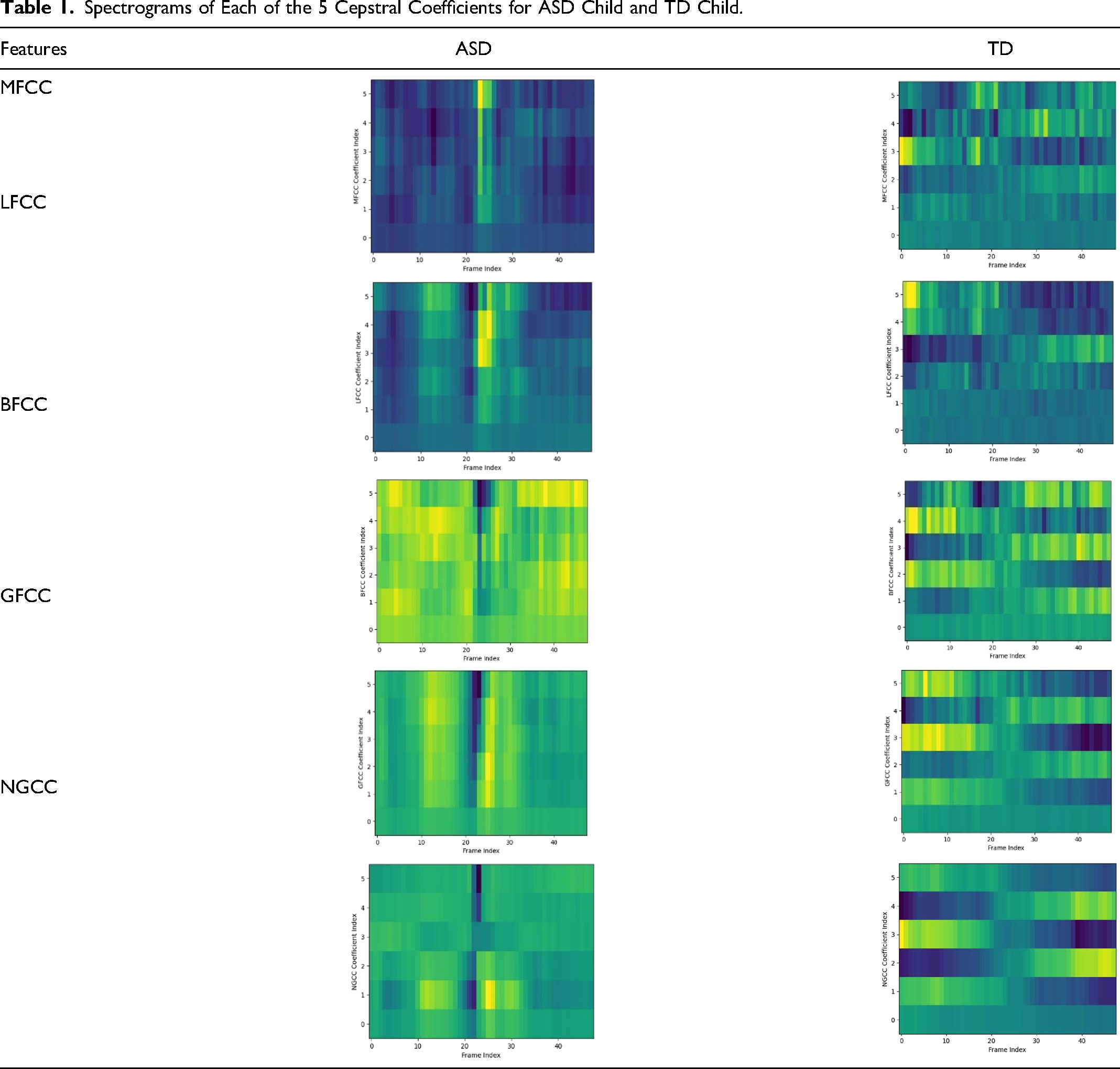
NGCC use normalized gammachirp filter bank can improve the accuracy of EEG analysis for tasks related to speech and music processing by combining the frequency selectivity of the gammatone filter bank with the temporal resolution of the chirplet transform, allowing for better detection and discrimination of spectral and temporal features in the EEG signal. The spectrograms of the MFCC, LFCC, BFCC, GFCC, and NGCC are the input data on which the neural networks will be trained. A spectrogram is used to represent a signal's intensity graphically with frequency on the X-axis and time on the Y-axis. It is plotted by dividing the signal into small segments of equal length such that there is no significant shift in the frequency over time in each segment. The colors and brightness in it reflect the signal strength. The brightness of color directly correlates with the signal's energy. Table 1 depicts the spectrograms of each of the 5 cepstral coefficients for ASD child and TD child.

Table 1.

Spectrograms of Each of the 5 Cepstral Coefficients for ASD Child and TD Child.

Features	ASD	TD
MFCC
LFCC
BFCC
GFCC
NGCC

Data Preparation

For extracting the abovementioned coefficients, a spatiotemporal approach was used. Eight different channels of the EEG namely O1, O2, T7, T8, F4, F3, F7, and F8 from 3 different brain lobes: Occipital, Central, and Temporal were considered for data acquisition. The cepstral coefficients are determined for every 1000 samples. The key advantage of this method is that a holistic and overall image of the brain's response to the given stimuli is obtained, and the classification of ASD and TD will be done based on this more overall image rather than specific channels. There were totally 20 subjects; 10 of TD children, and 10 of children with Autism.

Model Training

This paper investigates and analyses some of the current cutting-edge architectures in deep neural networks, such as AlexNet, VGG16, and ResNet50 for the effective identification of ASD. In general, EEG spectrograms are complex images because they represent the frequency content of the EEG signals over time and it require networks with a large receptive field and the ability to learn complex features. AlexNet, VGG16, and ResNet50 have large receptive fields and the ability to learn complex features, making them suitable for EEG spectrogram classification.

The large receptive field allows the network to capture information from a broad range of frequencies and time points, enabling it to extract meaningful features from the spectrogram. Additionally, the ability to learn complex features allows the network to capture the complex relationships between different frequencies and time points in the spectrogram. AlexNet consists of 5 convolutional layers followed by max-pooling layers and 3 fully connected layers. It has a relatively small number of parameters, making it computationally efficient. VGG16 has a simple architecture, with a series of convolutional layers followed by max-pooling layers and 3 fully connected layers. The small filters used in the convolutional layers enable it to capture fine-grained details in the input image. The residual connections in ResNet50 enable it to learn more complex features and deeper representations, which are beneficial for tasks that require more complex representations. This paper also proceeds to attempt and improve the classification accuracy of the best classification model among the above by tweaking its architecture.

AlexNet

AlexNet is a popular deep CNN architecture in the 2012 ImageNet ILSVRC 2012 Competition.24 AlexNethas 22 layers with 60 million parameters, and the activation function is a Rectified Linear Unit. This architecture was altered to identify an input as just 2 classes instead of 1000 and was trained from the ground up using our own datasets. Before feeding the spectrograms into the network for training, they were reduced to 227 × 227 pixels. Lastly, in the output layer, a 2-way softmax activation function was used for classification.

VGG16

VGG16 has a total of 21 layers, out of which 16 only are weight layers, that is, learnable parameters layers.25 The authors of this model evaluated the networks and increased the depth with a small (3 × 3) convolution filter architecture, which showed a substantial improvement over some other state-of-the-art configurations. All layers except the final dense layer used Rectified Linear Unit activation, which was altered to identify just 2 classes. Before feeding the spectrograms into the network for training, they were reduced to a dimension of 224 × 224.

ResNet50

ResNet (short for Residual Networks) is a classic neural network that forms the basis for many applications of computer vision. ResNet50 model won the ImageNet challenge 2015. Prior to ResNet, training very deep neural networks was difficult because of the vanishing gradients problem, which impacted the model's convergence. ResNet employs skip connections that can skip certain layers, to resolve this.²⁶

Proposed Network

Since AlexNet was giving the best results for our dataset, it was modified in different ways to try and increase its accuracy with minimal loss. Extra convolutional layers were added, their orders changed, pooling styles changed, the optimizer changed, and the learning rate tweaked, all of which are discussed in detail in the results and discussion. Ultimately, one specific combination of these tweaks resulted in a testing accuracy of 90%. The tweak consists of 2 additional 2D convolutional layers. The convolution layers ensure that further deeper features are extracted and cost function used here was the categorical cross entropy function. The proposed architecture is presented in Figure 3.

Figure 3.

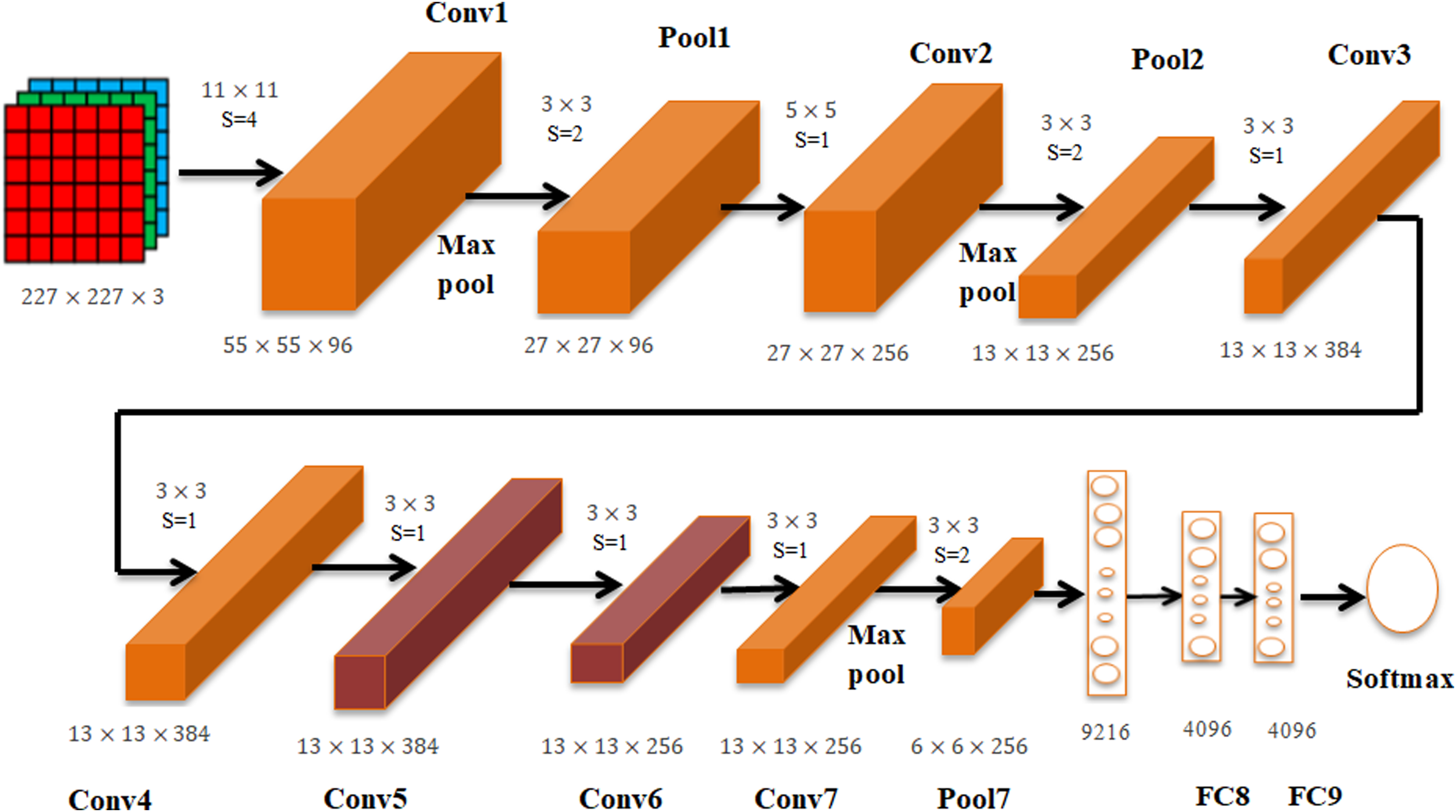
Architecture of the customized AlexNet.

Results and Discussion

Several experiments were carried out on the input dataset to measure the performance of the DL models, and this section summarizes the outcomes.

Environment Setup and Design

The training and evaluation were entirely done on Google Colab running Python 3 on the Google Compute Engine backend. The models were developed using the Keras library. The dataset was divided into 2 nonoverlapping sets, split into an 80:20 ratio for training and testing, respectively.

Evaluation Metrics

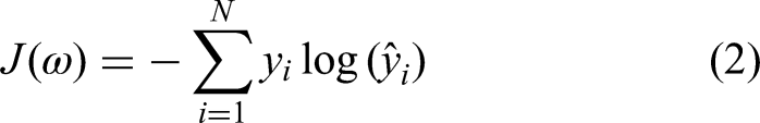
The network performance was evaluated on the basis of testing accuracy and testing loss. Having a low accuracy but a high loss indicates that the model makes significant errors in the majority of the data. If both loss and accuracy are low, it indicates that the model makes small errors in the majority of the data. If they are both high, it causes significant errors in some of the data. Finally, if the accuracy is high and the loss is low, the model makes minor errors on only a subset of the data, which is the ideal case. Hence, the best model was simply the one that gave maximum accuracy with minimum loss. To calculate the loss, a loss or cost function is used. For both the original AlexNet and the customized version of AlexNet this study has introduced, the cost function used here was the sparse categorical cross entropy function. For VGG16 and ResNet50, a binary cross entropy function was used. The relations for both the loss functions are presented in equations (1) and (2):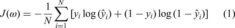

J (ω) = - \frac{1}{N} \sum_{i = 1}^{N} [y_{i} \log ({\hat{y}}_{i}) + (1 - y_{i}) \log (1 - {\hat{y}}_{i})]

(1)

J (ω) = - \sum_{i = 1}^{N} y_{i} \log ({\hat{y}}_{i})

(2)

Experimental Analysis

The training and testing process for the various DL models was evaluated in terms of accuracy and loss. The DL models were trained for 50 epochs, adjusted according to the timeout restrictions for Google Colab. To keep the training duration within and around an ample 2 h, the number of epochs for each network was changed accordingly. Table 2 summarizes the observations of performance metrics (accuracy) for the various DL models.

Table 2.

A Comparison of Performance Metrics for the Various Deep Learning Models.

Method	Accuracy (%)
Method	MFCC	LFCC	BFCC	GFCC	NGCC
AlexNet	0.7031	0.8516	0.6797	0.8203	0.7734
ResNet50	0.6609	0.7356	0.6839	0.6724	0.8448
VGG16	0.50	0.50	0.50	0.50	0.50
Customized AlexNet	0.800	0.9012	0.7500	0.8125	0.8750

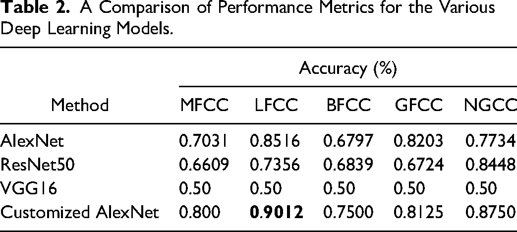
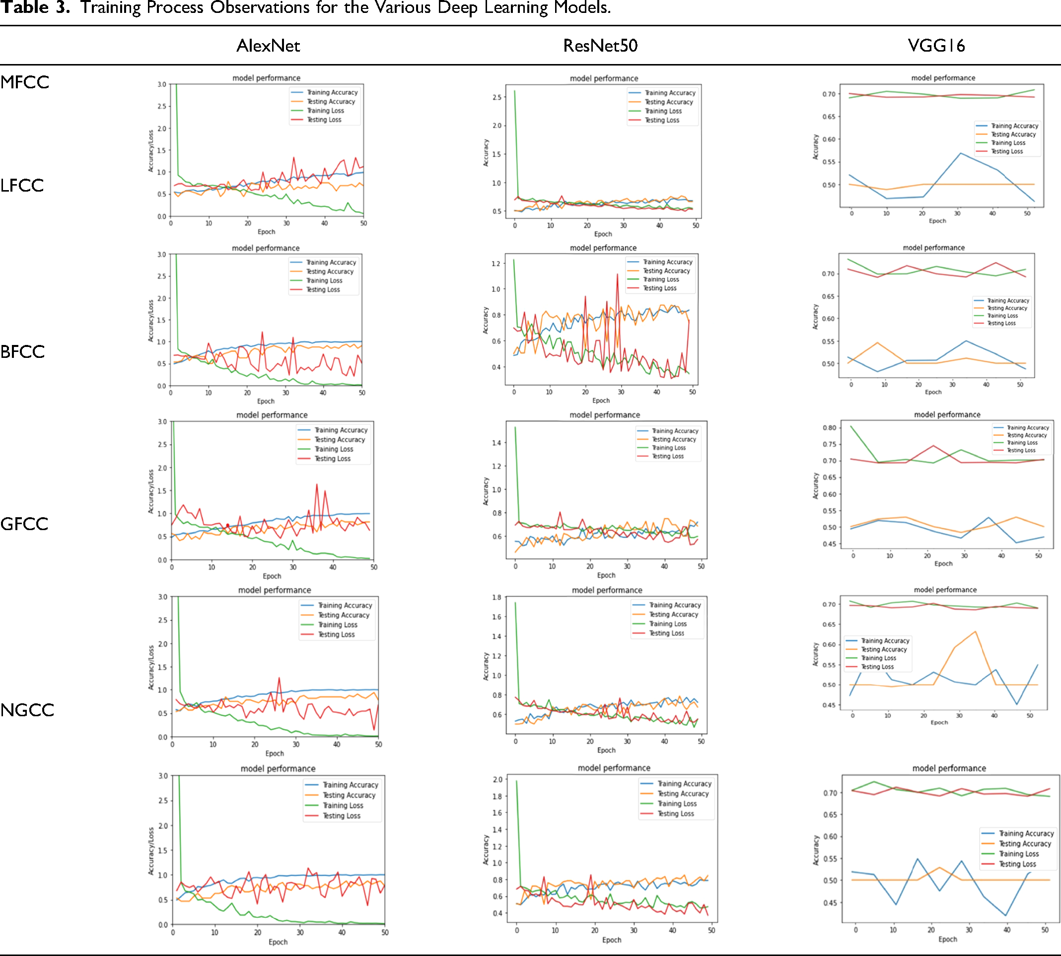
From Table 2, notice that AlexNet predicting for LFCC gave the best results for this short training time, with an accuracy of 85.16% and a loss of 0.3480. ResNet50 gave average or poor results for every Cepstral Coefficient except NGCC. Since it has 50 layers, training could take hours, especially from the ground up. Hence, transfer learning was applied, where the weights of the initial layers were imported directly from training for a different binary classification task, and only the deeper layers were trained for the task at hand. Training the model from scratch could possibly has given better results but at the expense of a much longer training time. VGG16 gave a low testing accuracy of 50%. Table 3 shows a graphical representation of the epochs versus model accuracy and loss.

Table 3.

Training Process Observations for the Various Deep Learning Models.

	AlexNet	ResNet50	VGG16
MFCC
LFCC
BFCC
GFCC
NGCC

Performance Analysis

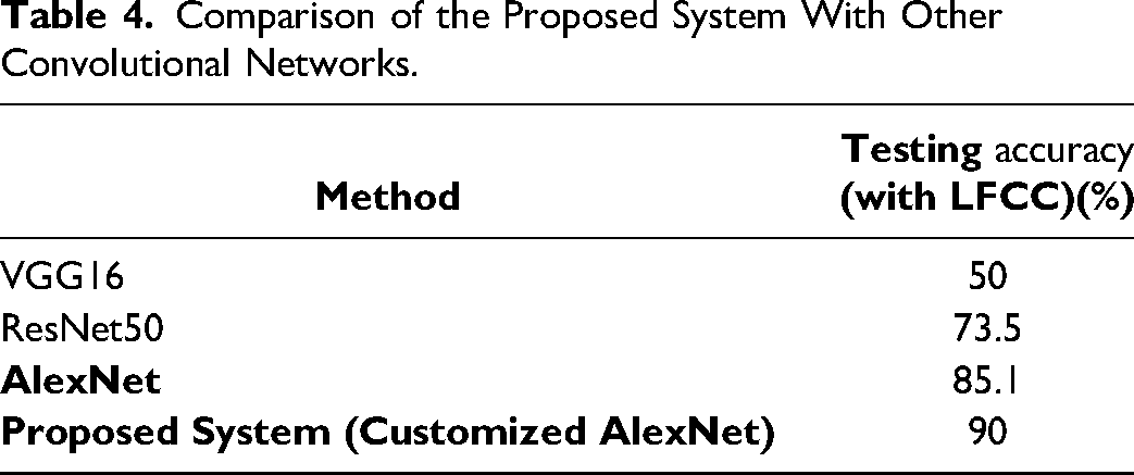
Table 4 depicts the comparison of the proposed system with other convolutional networks. Cepstral coefficients are used to extract the spectral information from the EEG signal. Cepstral coefficients spectrogram is used as input to CNN to improve the accuracy of discriminating the ASD and TD. Table 5 depicts the comparison of the proposed work with existing methods.

Table 4.

Comparison of the Proposed System With Other Convolutional Networks.

Method	Testing accuracy (with LFCC)(%)
VGG16	50
ResNet50	73.5
AlexNet	85.1
Proposed System (Customized AlexNet)	90

Table 5.

Comparison of the Proposed Method With Existing Methods.

Sources	Classifier	Accuracy (%)
Ali²⁷	CNN	80
Radhakrishnan et al²⁸	ResNet50	81
Mohi-ud-Din and Jayanthy²⁹	SqueezeNet, SVM	82
Proposed method	Customized AlexNet	90

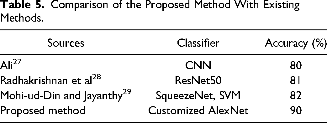
Ali acquired every second data and converted into 16 × 256 2D array, this is used to training CNN. Radhakrishnan et al used spectrogram to train ResNet50 for classification. Mohid-ud-Din et al used Scalograms (224 × 224 × 3) and extract deep features by squeezeNet and fed to training the SVM. All the above methods achieved accuracy in the range of 80–82%. Tahwid et al applied STFT throughout the signal is windowed at constant interval. This spectrogram is used for training their customized CNN model through this method achieved accuracy of 99.15% computational complexity will be high with STFT. In the proposed system with cepstral coefficients, 90% accuracy was achieved.

Conclusion

This paper proposes a DL system for the accurate diagnosis of ASD. The primary goal of this study is to evaluate the performance of state-of-the-art deep convolutional networks in the detection of ASD from EEG signals and to improve the best-performing network to give better accuracy by tweaking the architecture. Comprehensive study was conducted using various deep architectures such as AlexNet, VGGNet, and ResNet, and this is the first study that we are aware of, that optimizes a deep network by altering its architecture, following a quantitative research of the deep architectures stated above for ASD detection. Results of various experiments conducted show that the proposed system, a modified version of the AlexNet deep CNN model, outperforms the other models in detecting ASD from spectrograms of cepstral coefficients, with a maximum classification accuracy of 90%. The performance of the proposed network can be further improved by the application of multimodal sensory signals and other architectural customizations.

Footnotes

Authors’ Note

The study was conducted according to the guidelines of the Declaration of Helsinki and approved by the Institutional Ethics Committee of Sri Ramachandra Institute of Higher Education and Research.

Acknowledgments

The authors would like to thank Sri Ramachandra Institute of Higher Education and Research for providing the dataset used in this research work.

Declaration of Conflicting Interests

The author(s) declared no potential conflicts of interest with respect to the research, authorship, and/or publication of this article.

Funding

The author(s) received no financial support for the research, authorship, and/or publication of this article.

ORCID iD

R. Menaka

S. Saranya

References

Rutter

. Autism research: Prospects and priorities. J Autism Dev Disord. 1996;26(2):257-275. doi:10.1007/BF02172023

Nur Syahindah Husna

Syafeeza

Abdul Hamid

Wong

Atikah Raihan

. Functional magnetic resonance imaging for autism spectrum disorder detection using deep learning. Jurnal Teknologi. 2021;83(3):45-52. doi:10.11113/jurnalteknologi.v83.16389

Buescher

AVS

Cidav

Knapp

Mandell

. Costs of autism spectrum disorders in the United Kingdom and the United States. JAMA Pediatr. 2014;168(8):721. doi:10.1001/jamapediatrics.2014.210

Raina

. Need for autism spectrum disorder research in India. Med J DY Patil Vidyapeeth. 2021;14(4):432-433. doi:10.4103/mjdrdypu.mjdrdypu_416_20

Maddox

Rump

Stahmer

, et al. Concordance between a U.S. Educational autism classification and the autism diagnostic observation schedule. J Clin Child Adolesc Psychol. 2020;49(4):469-475. doi:10.1080/15374416.2019.1567345

Seltzer

Krauss

Shattuck

Orsmond

Swe

Lord

. The symptoms of autism spectrum disorders in adolescence and adulthood. J Autism Dev Disord. 2003;33(6):565-581. doi:10.1023/B:JADD.0000005995.02453.0b

Magaña

Vanegas

. Diagnostic utility of the ADI-R and DSM-5 in the assessment of Latino children and adolescents. J Autism Dev Disord. 2017;47(5):1278-1287. doi:10.1007/s10803-017-3043-2

Brentani

Paula

Bordini

, et al. Autism spectrum disorders: an overview on diagnosis and treatment. Rev Bras Psiquiatr. 2013;35(suppl 1):S62-S72. doi:10.1590/1516-4446-2013-S104

Khodatars

Shoeibi

Sadeghi

, et al. Deep learning for neuroimaging-based diagnosis and rehabilitation of autism spectrum disorder: a review. Comput Biol Med. 2021;139:104949. doi:10.1016/j.compbiomed.2021.104949

10.

Meedeniya

Rubasinghe

. A review of supportive computational approaches for neurological disorder identification. In: Wadhera

Kakkar

, eds. Advances in Medical Diagnosis, Treatment, and Care. IGI Global; 2020:271-302. doi:10.4018/978-1-7998-3069-6.ch016

11.

Brihadiswaran

Haputhanthri

Gunathilaka

Meedeniya

Jayarathna

. EEG-based processing and classification methodologies for autism spectrum disorder: a review. J Comput Sci. 2019;15(8):1161-1183. doi:10.3844/jcssp.2019.1161.1183

12.

Boutros

Lajiness-O’Neill

Zillgitt

Richard

Bowyer

. EEG changes associated with autistic spectrum disorders. Neuropsychiatr Electrophysiol. 2015;1(1):3. doi:10.1186/s40810-014-0001-5

13.

Chawla

Rana

Kaur

Singh

. Computer-aided diagnosis of autism spectrum disorder from EEG signals using deep learning with FAWT and multiscale permutation entropy features. Proc Inst Mech Eng H. 2023;237(2):282-294. doi:10.1177/09544119221141751

14.

Abdolzadegan

Moattar

Ghoshuni

. A robust method for early diagnosis of autism spectrum disorder from EEG signals based on feature selection and DBSCAN method. Biocybern Biomed Eng. 2020;40(1):482-493. doi:10.1016/j.bbe.2020.01.008

15.

Haputhanthri

Brihadiswaran

Gunathilaka

, et al. An EEG based Channel Optimized Classification Approach for Autism Spectrum Disorder. In: 2019 Moratuwa Engineering Research Conference (MERCon). IEEE; 2019:123-128. doi:10.1109/MERCon.2019.8818814.

16.

Haputhanthri

Brihadiswaran

Gunathilaka

, et al. Integration of facial thermography in EEG-based classification of ASD. Int J Autom Comput. 2020;17(6):837-854. doi:10.1007/s11633-020-1231-6

17.

Mohanta

Mukherjee

Mirtal

. Acoustic Features Characterization of Autism Speech for Automated Detection and Classification. In: 2020 National Conference on Communications (NCC). IEEE; 2020:1-6. doi:10.1109/NCC48643.2020.9056025.

18.

Cooney

Folli

Coyle

. Mel Frequency Cepstral Coefficients Enhance Imagined Speech Decoding Accuracy from EEG. In: 2018 29th Irish Signals and Systems Conference (ISSC). IEEE; 2018:1-7. doi:10.1109/ISSC.2018.8585291.

19.

Tawhid

MNA

Siuly

Wang

. Diagnosis of autism spectrum disorder from EEG using a time–frequency spectrogram image based approach. Electron Lett. 2020;56(25):1372-1375. doi:10.1049/el.2020.2646

20.

Tawhid

Siuly

Wang

Whittaker

Wang

Zhang

. A spectrogram image based intelligent technique for automatic detection of autism spectrum disorder from EEG. Mumtaz W, ed. PLoS One. 2021;16(6):e0253094. doi:10.1371/journal.pone.0253094

21.

Baygin

Dogan

Tuncer

, et al. Automated ASD detection using hybrid deep lightweight features extracted from EEG signals. Comput Biol Med. 2021;134:104548. doi:10.1016/j.compbiomed.2021.104548

22.

Nogay

Adeli

. Machine learning (ML) for the diagnosis of autism spectrum disorder (ASD) using brain imaging. Rev Neurosci. 2020;31(8):825-841. doi:10.1515/revneuro-2020-0043

23.

World Medical Association. World Medical Association declaration of Helsinki. Ethical principles for medical research involving human subjects. Bull World Health Organ. 2001;79(4):373-374. PMID: 11357217; PMCID: PMC2566407.

24.

Krizhevsky

Sutskever

Hinton

. ImageNet classification with deep convolutional neural networks. Commun ACM. 2017;60(6):84-90. doi:10.1145/3065386

25.

Qassim

Verma

Feinzimer

. Compressed residual-VGG16 CNN model for big data places image recognition. In: 2018 IEEE 8th Annual Computing and Communication Workshop and Conference (CCWC). IEEE; 2018:169-175. doi:10.1109/CCWC.2018.8301729.

26.

Zhang

Ren

Sun

. Deep Residual Learning for Image Recognition. In: 2016 IEEE Conference on Computer Vision and Pattern Recognition (CVPR). IEEE; 2016:770-778. doi:10.1109/CVPR.2016.90.

27.

Ali

. Autism spectrum disorder classification on electroencephalogram signal using deep learning algorithm. Int J Artif Intellig. 2020;9(1):91. doi:10.11591/ijai.v9.i1.pp91-99

28.

Radhakrishnan

Ramamurthy

Choudhury

Won

Manoharan

. Performance analysis of deep learning models for detection of autism Spectrum disorder from EEG signals. TS. 2021;38(3):853-863. doi:10.18280/ts.380332

29.

Mohi-ud-Din

Jayanthy

. Detection of Autism Spectrum Disorder from EEG signals using pre-trained deep convolution neural networks. In: 2021 Seventh International Conference on Bio Signals, Images, and Instrumentation (ICBSII). IEEE; 2021:1-5. doi:10.1109/ICBSII51839.2021.9445193.

An Improved AlexNet Model and Cepstral Coefficient-Based Classification of Autism Using EEG

Abstract

Keywords

Introduction

Related Works

Proposed System

Data Acquisition

Stimuli selection

Preprocessing

Feature Extraction

Data Preparation

Model Training

AlexNet

VGG16

ResNet50

Proposed Network

Results and Discussion

Environment Setup and Design

Evaluation Metrics

Experimental Analysis

Performance Analysis

Conclusion

Footnotes

Authors’ Note

Acknowledgments

Declaration of Conflicting Interests

Funding

ORCID iD

References