Evaluating ship-to-shore schedules using simulation

Abstract

During military operations in coastal regions, resources, such as personnel and vehicles, are brought from large amphibious ships to the shore using smaller ships and helicopters. The aim is to transport these resources as fast as possible while adhering to different types of constraints. This is called the ship-to-shore problem and has been solved assuming deterministic parameters regarding the speed and (un)loading time of the connectors. These schedules might therefore not be robust to delays. We developed a simulation model to analyze the effect of uncertainty in these parameters on the execution of a schedule. We analyze (1) whether these discrete time periods are able to capture the delays, (2) the effect of using more conservative parameters when constructing a schedule, and (3) the effect of being less rigid in the execution, i.e., when being allowed to depart a limited time ahead of schedule. We find that significant delays occur and that using more conservative parameters for the (un)loading time can have a positive significant effect on the duration of the operation. Being less rigid can also have a positive significant effect on the duration; however, it comes at the cost of violating constraints regarding the grouped delivery of resources.

1. Introduction

During military operations in coastal regions, resources are brought from large amphibious ships to the shore using smaller ships and helicopters, called connectors. It is essential to carry out the transportation of the resources efficiently to facilitate the earliest possible start of the tasks on land. Hence, the aim is to schedule the connector trips to the shore such that the makespan, the duration of the operation, is minimized. Therefore, the need for a fast algorithm to construct a schedule for this transportation problem arises. This problem is called the ship-to-shore problem, of which variations have been studied.^1–5

In the ship-to-shore problem, the aim is to find, for each connector, a route that should be executed such that the makespan is minimized. A route defines a set of round-trips between a sea base (SB) and a landing area (LA) location that should be executed as well as the resources that should be transported in each trip. Based on interviews with experts at the Defence, Safety and Security unit of the Netherlands Organisation for Applied Scientific Research (TNO), we have identified various constraints that have to be adhered to in a schedule. These can be split into constraints regarding the connectors, the delivery of the resources to the shore, and the (un)loading of the resources.

Connectors have a space and weight capacity that determines what set of resources can be simultaneously transported. There can be specific limitations in the way connectors can be loaded, e.g., the load of the connector should be balanced and resources might have to be secured which can only be done at limited spots, restricting the number of ways connectors can be loaded. Furthermore, the connectors have a fuel capacity and might therefore have to be refueled at an SB. The speed of a connector can be dependent on the weight of the load on the connector.

Resources have different priority levels that determine a partial ordering of the delivery of resources to the shore. Here, a strict ordering exists where all resources with a higher priority should be delivered before resources with a lower priority are delivered. In addition, certain resources can belong to the same resource set and have to be delivered at the same time or closely after each other, called a resource set constraint. An example of a resource set is a unit that trained together plus the vehicles containing their personal supplies. To avoid the situation where either the vehicle or the personnel has to wait on the shore, we impose that these are delivered together or closely after each other. ⁶ The time interval in which resources from a resource set are delivered is called a delivery wave. Furthermore, at an SB and LB, a limited number of (un)loading spots are available. Hence, there is a limit on the number of connectors that can be (un)loaded at the same time.

Wagenvoort et al. ⁵ consider the ship-to-shore problem as described above and design an exact branch-and-price algorithm, as well as a greedy heuristic. Christafore, ¹ Danielson, ² Strickland, ³ and Villena ⁴ also study the ship-to-shore problem. Compared to Wagenvoort et al., ⁵ they do not consider all constraints regarding the coordination of the delivery of resources. Therefore, we use schedules constructed using the method of Wagenvoort et al. ⁵

Given a schedule for the ship-to-shore problem, preparations are made accordingly. This implies that switching the order of resources in which they are loaded is not always possible or leads to significant delays. ⁷ Once the resources are placed in a certain order on the large amphibious warfare ships, resources scheduled to be transported earlier may block other resources that are scheduled to be transported later. Furthermore, the schedule is communicated to the staff on the ship, and they make preparations accordingly. This prevents them from departing significantly before their planned departure time, as they are not ready for departure and might have other conflicting tasks. Therefore, when executing a schedule for the transport operation, the schedule is followed as closely as possible. However, travel times and (un)loading times are stochastic and weather conditions can be different than predicted, also affecting the travel times of the connectors. This means that delays can occur, which can propagate through the schedule, as the order in which the resources are loaded onto a connector is fixed when a schedule is executed and connectors are not allowed to depart ahead of time.

Research on the ship-to-shore problem has assumed deterministic parameters regarding the speed and the (un)loading time of the connectors. The resulting schedules might therefore not be robust for delays, and this can greatly affect the duration of the transportation of the resources. In general, adding slack to a schedule can help capture these delays and can therefore be beneficial for the realized makespan. One way to add slack is to schedule with more conservative parameters. However, adding too much slack, by being too conservative in the parameters, or by adding slack at the wrong moments, can negatively affect the realized makespan, as the order of the connectors is fixed and connectors cannot depart before their scheduled time.

Wagenvoort et al. ⁵ make use of a time-space network to model the ship-to-shore problem. The time-space network consists of nodes that correspond to a location at a certain discrete time period. Arcs connecting nodes correspond to transitions through both time and space. The inputs in Wagenvoort et al. ⁵ are deterministic, and the length of the discrete time period is set to the maximum (un)loading time of all connectors such that all connectors can be (un)loaded within one time period. Discrete time periods create buffer time in the schedule when a connector can (un)load faster or when the travel time between two locations is not equal to an integer multiple of the time period length. This buffer time could help capture delays. However, the buffer time occurs due to the design choice for the time-space network and is not incorporated as slack by the model to avoid delays. Therefore, it might not be sufficient to handle the delays, and it is of interest how well such a schedule performs.

We are therefore interested in the following questions:

• RQ1. How well does a schedule generated using discrete time periods perform when parameters are stochastic?

• RQ2. What is the trade-off between using a schedule constructed using more conservative parameters, and the realized makespan?

• RQ3. What is the effect of being less rigid in the execution of a schedule?

Simulation models can be used to model and evaluate the behavior of a system over time. ⁸ Therefore, they can be used to assess the robustness of a planning, as well as the effectiveness of new policies.^9–11 Simulation models can be particularly useful when limited data are available about the performance of a system, as is the case for the ship-to-shore problem which is usually only executed once. ¹²

Horne and Irony ¹³ use a simulation to analyze the trade-off between the number of connectors, (un)loading positions, and travel time between the SB and LA. They do, however, not consider different types of connectors that can use different (un)loading spots, priorities, and resource sets. We therefore develop a simulation model in which a schedule is given as input and its execution is evaluated given uncertainty in the speed and (un)loading time as well as changes in the predicted weather conditions that affect the travel time. The simulation model follows the schedule, by adhering to the order in which connectors are loaded at an SB, and by only allowing connectors to start a limited amount of time ahead of schedule. Furthermore, the simulation model considers the constraints that arise in the ship-to-shore problem.

We use the simulation model to analyze the performance of schedules constructed using the approach of Wagenvoort et al. ⁵ We find that uncertainty in the parameters has a significant effect on the performance of the schedule. Hence, the buffer time in the schedule arising from the discrete time periods does not suffice to capture these delays. In fact, on average, connectors arrive late in over 30% of their trips. Using a conservative schedule can improve the performance when a more conservative (un)loading time is used. However, using more conservative (un)loading times can produce worse results, especially when you are not interested in the average performance but a worst-case performance. Being less rigid in the execution by allowing connectors to depart a limited time ahead of schedule generally has a positive effect on the performance of the schedule. However, this comes at the cost of violating the resource set constraints.

The paper is organized as follows. We describe how we simulate the execution of a schedule and the types of uncertainties we consider in section 2. In section 3, we describe the set-up of the experiments. We report and discuss the results of the experiments in section 4 and give a conclusion in section 5.

2. Discrete-event simulation

We use a discrete-event simulation in which we take a schedule as input and model the movement of the connectors over time while incorporating uncertainty in deviations from the wind and current used in generating the schedules, the speed of the connectors, and the (un)loading time. The schedule specifies for each connector what trips it should make and thus when it should start (un)loading, when it should depart, and what it should carry in each trip from an SB to an LA. We model the movement of the connectors using the following events: Arrival at an SB, departure from an SB, arrival at an LA, departure from an LA. During the simulation, certain policies have to be adhered to while executing the schedule. In this section, we describe the types of uncertainty we consider in the simulation, the policies we have to adhere to, and the output of the simulation model. An overview of the procedure for each event is given in Appendix 1.

2.1. Uncertainty in the ship-to-shore problem

During the planning of the ship-to-shore problem, deterministic parameters are used, while in reality, these are stochastic. Furthermore, the weather conditions can differ from the expected weather conditions, affecting the speed of the connectors. In this section, we explain the types of uncertainty that arise in the execution of the ship-to-shore problem in more detail.

The speed of a connector is used to determine the required travel time between the locations. The speed can be constant or dependent on the weight of the load it carries. However, a connector does not always travel at maximum speed due to, e.g., small navigation errors or detours. This will result in a net speed slightly below the maximum speed. We therefore determine the net speed of a connector for each trip made by the connector according to a distribution that is input to the simulation.

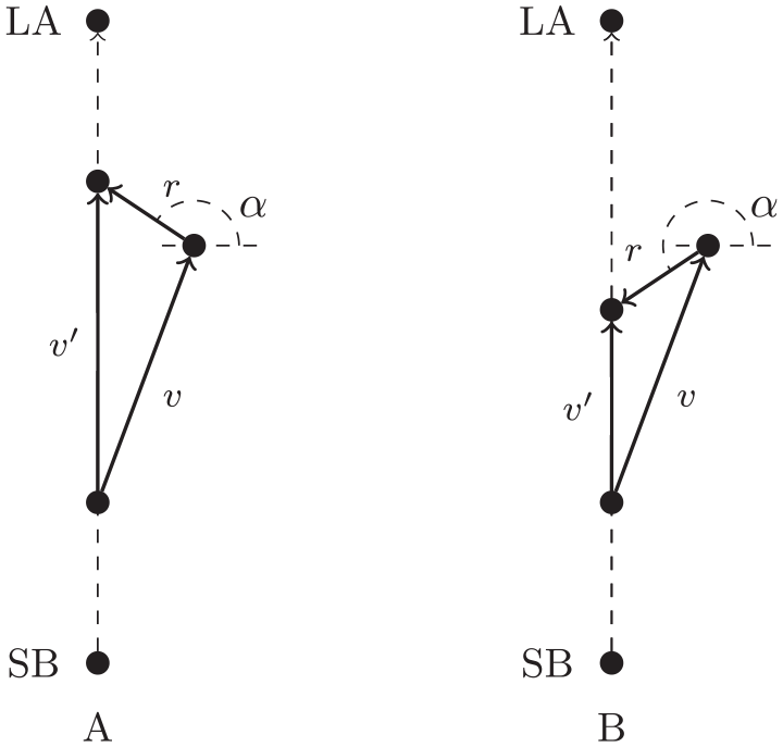
Furthermore, the travel time is dependent on the weather conditions. Namely, the current and/or wind affect the speed at which a connector travels. In the planning phase, the predicted water current and/or wind can be taken into account. However, the actual current or wind can be different. We consider a change in the current or wind as denoted by Figure 1. Namely, if a planning was made with the net speed and direction according to the predicted current/wind, and the actual current/wind deviates, the speed and direction will have to be adjusted according to the vector labeled as “adjustment” in Figure 1. This affects the travel time, as the connector has to adjust its direction for the change in the current/wind (see Example 1).

• Example 1. Two examples are given in Figure 2. Here, the angle of the change in the current and/or wind is denoted by $\alpha$ and the strength is $\mathrm{r}$ nautical miles. If the direction and strength of the current and/or wind are not taken into account, the connectors will not end up at the LA but to the left of it. Therefore, the connectors will have to steer to the right in order to arrive at the LA. The connector will thus travel at a speed $\mathrm{v}$ in the denoted direction and have a realized speed of $\mathrm{v}\prime$ toward the LA.

• This means that in case A, the realized speed $\mathrm{v}\prime$ is higher than the speed of the connector, and in case B, the realized speed $\mathrm{v}\prime$ is lower than the speed of the connector. When returning to the SB from the LA, the reverse will hold.

Figure 1.

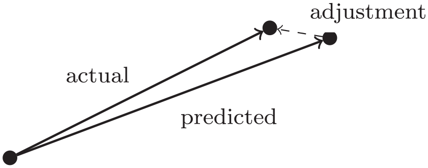
Vector representation of the effect of a change in the current/wind in direction compared to the predicted current/wind.

Figure 2.

Vector representation of the effect of a current or wind in direction $\alpha$ and with strength $r$ on the speed $v$ .

Besides changes in the speed of the connectors, changes in the (un)loading time of a connector at an SB/LB can occur. Delays in (un)loading are caused by small delays in placing or removing the resources on/from the connectors. Furthermore, small repairs and refueling can be done at the SB which could cause delays. At the LB, connectors can get stuck in sand and therefore take longer to depart the LB. Therefore, we determine the (un)loading time of a connector for each time it (un)loads according to a distribution that is input to the simulation.

2.2. Simulation policies

We consider the following simulation policies.

First, we adhere to the (un)loading order provided by the schedule. Due to the uncertainty in the simulation parameters, it is possible that a connector that is scheduled to (un)load at a later time than another connector arrives first. Preparations are made according to the schedule, e.g., at the SB, the resources are gathered that should be loaded onto the connector. In this case, the resources for the next loading should be gathered instead including personnel, which can result in additional delays. Furthermore, this could lead to violations of the priority or resource set constraints. Hence, a connector cannot be (un)loaded before the connectors that are scheduled to (un)load before have finished or started (un)loading.

Second, we limit the time the connectors can be ahead of schedule. For the same reasons as mentioned above, being far ahead of schedule can cause difficulties as preparations have not been completed yet. Therefore, we set a limit to how far ahead of schedule a connector can be (un)loaded.

Finally, we adhere to all constraints of the ship-to-shore problem, if possible. This implies that we adhere to the capacity constraints at the SBs and LAs. Namely, there is a maximum number of connectors that can be (un)loaded at the same time at an SB or LA. If a connector arrives and should be (un)loaded next, but all (un)loading spaces are occupied, the connector has to wait. In addition, some connectors are only compatible with certain (un)loading locations, and they are therefore not able to (un)load at a free spot that is not compatible. Furthermore, we adhere to the constraints regarding the ordering of resources. Namely, a strict priority ordering of the resources exists which implies that a connector carrying priority $\pi +1$ resources will wait until all priority $\pi$ resources are delivered. Finally, we adhere to the resource set constraints, if possible. These constraints ensure that resources that belong to the same resource set are delivered at the same time or closely after each other. Hence, if it is known in advance that a connector taking part in a delivery wave is delayed, the start of the wave will be postponed. However, it is possible that a connector taking part in a delivery wave experiences a delay when another connector is already delivering resources from that wave. In that case, the wave might be violated, and we consider this a violation of the resource set constraint.

2.3. Output of the simulation model

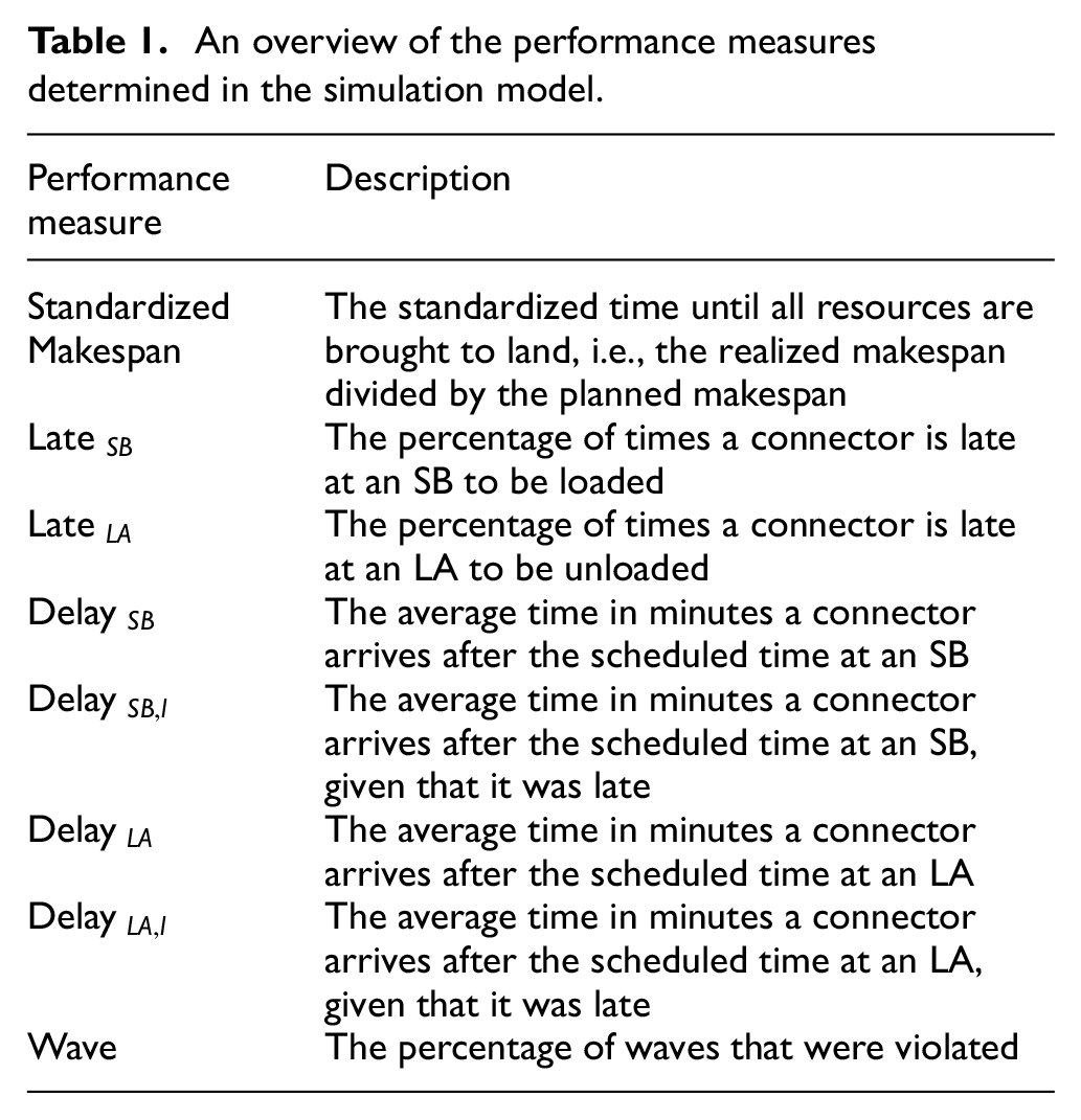
Our main interest is the realized makespan when executing a schedule with stochastic parameters. Besides the makespan, we also determine, from the simulation, the percentage of time a connector is late for loading at an SB and the percentage of time a connector is late for delivery at the LA. In addition, we determine the average delay at an SB or at an LA. Finally, since resource set constraints might be violated, we determine the percentage of delivery waves that are violated. We consider a delivery wave violated when the time between the completion of a delivery till the time of the start of the next delivery of that resource set differs by more than the length of one discrete time period. An overview of the performance measures we consider is given in Table 1.

Table 1.

An overview of the performance measures determined in the simulation model.

Performance measure	Description
Standardized Makespan	The standardized time until all resources are brought to land, i.e., the realized makespan divided by the planned makespan
${\mathrm{Late}}_{\mathrm{SB}}$	The percentage of times a connector is late at an SB to be loaded
${\mathrm{Late}}_{\mathrm{LA}}$	The percentage of times a connector is late at an LA to be unloaded
${\mathrm{Delay}}_{\mathrm{SB}}$	The average time in minutes a connector arrives after the scheduled time at an SB
${\mathrm{Delay}}_{\mathrm{SB},l}$	The average time in minutes a connector arrives after the scheduled time at an SB, given that it was late
${\mathrm{Delay}}_{\mathrm{LA}}$	The average time in minutes a connector arrives after the scheduled time at an LA
${\mathrm{Delay}}_{\mathrm{LA},l}$	The average time in minutes a connector arrives after the scheduled time at an LA, given that it was late
Wave	The percentage of waves that were violated

3. Experimental design

In this section, we describe the design of our experiments. We first describe the distributions we use for the different parameters. Then, we describe which experiments and tests we perform to answer our research questions.

3.1. Simulation parameters

Input for the simulation are the distributions for the stochastic parameters defined in section 2. Here, we determine the change in the current/wind at the start of each replication, i.e., this effect is fixed within a replication. The travel time and (un)loading time uncertainty are considered for each individual trip and (un)loading activity. The distribution of the change in current/wind and the speed and (un)loading time is an input to the simulation and can thus be varied. We consider the following distributions in our experiments.

For the change in the current/wind, we consider a direction as an angle, $\alpha$ , and speed in nautical miles, $r$ , as given in Figure 3. Here, we take $\alpha ~U(0,360)$ degrees and $r~U(0,1)$ nautical miles. This implies that each direction is equally likely to occur as well as each speed up to one nautical miles.

Figure 3.

Change in the current/wind.

For the speed of the connectors, we consider a deviation from the maximum speed. In other words, the speed the connector has during a trip is equal to $s(1-x)$ , where $s$ is the maximum speed of the connector and $x$ a realization of $X~f_X\left(x\right)=4\cos \left(4\pi x\right)+4$ for $0\le x\le 0.25$ . This implies that a connector will have a speed of at least 75% of its maximum speed. Furthermore, small reductions in the speed are likely, while large reductions in the speed are unlikely. The distribution of the reduction in the speed is given in Figure 4(a).

Figure 4.

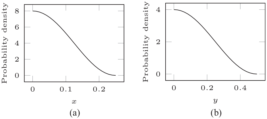
Simulation parameter data: (a) Distribution for the speed uncertainty. (b) Distribution for the loading uncertainty.

For the (un)loading time of the connectors, we consider an addition to the minimum required (un)loading time. In other words, the time it takes for the connector to be (un)loaded is equal to $t(1+y)$ , where $t$ is the minimum required time and $y$ a realization of $Y~f_Y\left(y\right)=2\cos \left(2\pi y\right)+2$ for $0\le y\le 0.5$ . This implies that a connector will take at most 1.5 times its minimum required time to be (un)loaded. Furthermore, small increases in the time are likely, while large increases in the time are unlikely. The distribution of the additional time is given in Figure 4(b).

To make a fair comparison between the simulation output of different schedules, we use different streams of random numbers. Namely, we use one stream of random numbers to determine the deviation of the wind and current, such that the $n^{\mathrm{th}}$ replication of each simulation has the same weather conditions. Furthermore, we specify for each connector two separate streams of random numbers, one for the travel times and one for the (un)loading times.

3.2. Experiments

In the simulation model, we take a schedule as input. We then simulate the execution of the schedule according to the policies defined in section 2.2 and the distribution for the parameters in section 3.1 for 100,000 replications.

To answer our first research question, we analyze the performance of a schedule constructed using discrete time periods. We therefore compare the simulation output with the planned makespan using a t-test. We analyze the performance with respect to the makespan, the percentage of times a connector is late to (un)load, the average delay when (un)loading, and the percentage of times a wave is violated.

To test the performance of the schedule with respect to the makespan, we test whether the average realized makespan deviates significantly from the planned makespan. Hence, we test the null hypothesis $H_0:\overline{X}=X_0$ against the alternative hypothesis $H_1:\overline{X}>X_0$ using a one-sided t-test. Here, $X_0$ is the planned makespan and $\overline{X}$ is the average makespan obtained from the simulation model. To test the performance of the schedule with respect to delays and wave violations, we test whether the average of the metric deviates significantly from 0 and thus use the above-described one-sided t-test with $X_0=0$ and $\overline{X}$ the average value of the corresponding metric.

Our second research question relates to the trade-off between using more conservative parameters and using the most optimistic parameters in the construction of a schedule. We therefore generate schedules using more conservative parameters by running the branch-and-price algorithm from Wagenvoort et al. ⁵ using these more conservative parameters for the speed of the connectors or for the (un)loading times. We then simulate the execution of these schedules and compare them to the simulated performance of the base schedule, i.e., the schedule created using the maximum speeds and (un)loading times equal to the maximum (un)loading time of all connectors. We test whether these differ significantly from each other using a paired t-test. This test is possible as the samples are dependent due to the usage of different streams of random numbers for different purposes. For example, each $i^{\mathrm{th}}$ replication has the same weather conditions because these are generated using a separate stream of random numbers.

Let $X_1$ and $X_2$ denote the samples of the execution of the two schedules. Let $x_i=x_{1i}-x_{2i}$ be the difference of pair $i$ between sample 1 and 2 and ${\overline{X}}_D$ the average of the difference between the pairs. As we are interested in whether the samples are significantly different, we define the null hypothesis $H_0:{\overline{X}}_D=0$ and the alternative hypothesis $H_1:{\overline{X}}_D\ne 0$ and apply the paired t-test.

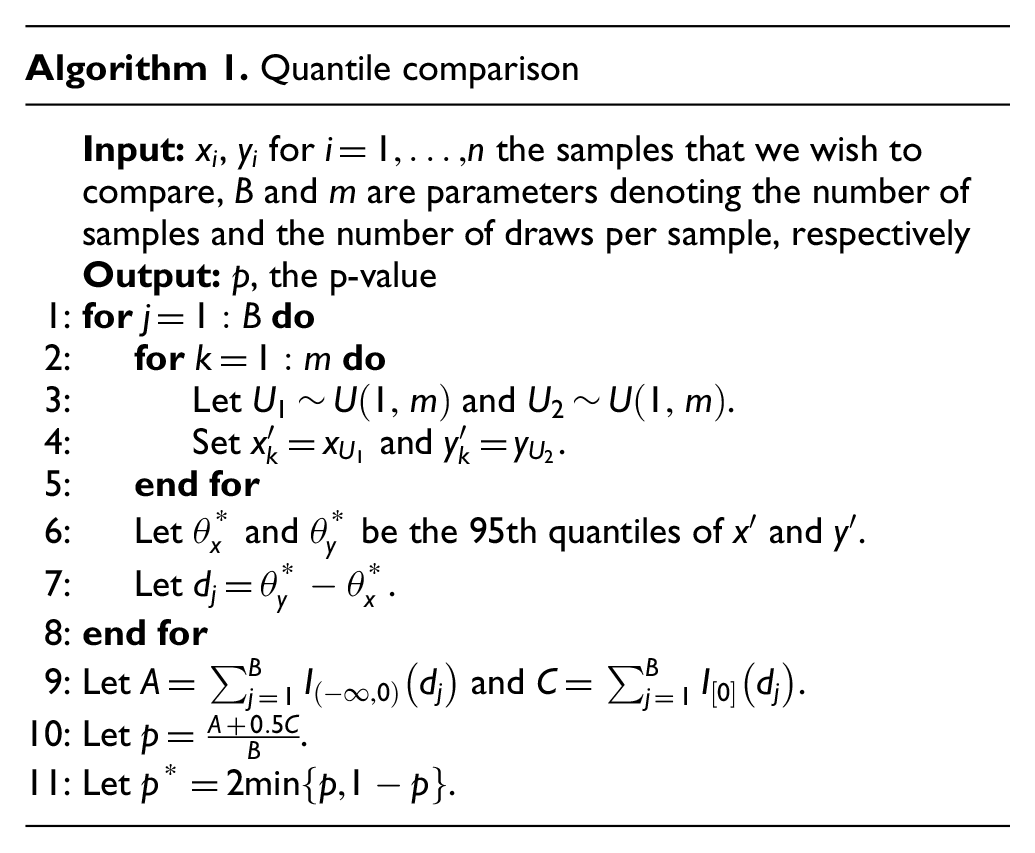
However, in the paired t-test, we compare the averages with each other, while the schedule is only executed once and we thus do not observe the average realized makespan when executing a schedule in practice. We therefore additionally consider a quantile comparison to see whether the schedules perform significantly different at the 95th percentile. We follow the approach of Wilcox et al. ¹⁴ to determine whether the 95th percentiles of two samples are significantly different (see Algorithm 1). In this test, random samples are generated from each original sample, and the difference between the 95th percentile in each of the paired samples is determined. Then, the one-sided p-value is determined by counting the number of times the difference is negative or equal. We do this based on $B=2000$ draws and samples of size $m=1,000,000$ . The generalized p-value, $p^{*}$ , can then be determined as $p^{*}=2\min \{p,1-p\}$ and can be used for a two-sided test.

Algorithm 1. Quantile comparison

Input: $x_i$ , $y_i$ for $i=1,\dots ,n$ the samples that we wish tocompare, $B$ and $m$ are parameters denoting the number ofsamples and the number of draws per sample, respectively  Output: $p$ , the p-value 1: for $j=1:B$ do 2:  for $k=1:m$ do 3:   Let $U_1~U(1,m)$ and $U_2~U(1,m)$ . 4:   Set $x_k\prime =x_{U_1}$ and $y_k\prime =y_{U_2}$ . 5:  end for 6:  Let ${\theta }_x^{*}$ and ${\theta }_y^{*}$ be the 95th quantiles of $x\prime$ and $y\prime$ . 7:  Let $d_j={\theta }_y^{*}-{\theta }_x^{*}$ . 8: end for 9: Let $A=\sum _{j=1}^B{I}_{(-\infty ,0)}\left(d_j\right)$ and $C=\sum _{j=1}^B{I}_{[0]}\left(d_j\right)$ . 10: Let $p=\frac{A+0.5C}{B}$ . 11: Let $p^{*}=2\min \{p,1-p\}$ .

The final research question relates to the effect of being less rigid in the execution of a schedule. Therefore, we give an additional input to the simulation model defining how many minutes a connector is allowed to be ahead of schedule. We simulate the execution of each schedule while being allowed to be $x\in \{10,30,60\}$ min ahead of schedule. We then compare the performance of these schedules with the execution of the schedule with $x=0$ . We perform both the paired t-test and the quantile comparison on the samples similarly as for the second research question.

4. Results

In this section, the results of our simulation model are presented, where a 5% significance level is used for all tests. The experiments are conducted using 15 instances, of which the data are provided by the Royal Netherlands Navy. The instances all have multiple SBs and LAs that are 15 nautical miles apart. There are four to six connectors available in each instance. The number of resources that are transported during the operation ranges from 20 to 244 items and varies from people to large vehicles. These resources are transported in up to 15 trips taking between 6.5 and 20 h.

The schedules are generated using deterministic values. However, the conditions during the execution of the schedule can vary as described in section 2.1. Therefore, we perform two experiments. In both experiments, schedules are constructed using deterministic parameters. In the first experiment, we use a schedule constructed using the most optimistic parameters, namely the maximum speed and minimum (un)loading time, which we call the base schedule. We then analyze the effect of stochastic parameters when executing the base schedule using the simulation. In the second experiment, we use more conservative parameters for the speed or (un)loading time to construct a schedule. We then compare the simulation output of these schedules with the simulation output of the base schedule to analyze the effect of using more conservative parameters in the schedule construction. Finally, we analyze the effect of being less rigid in executing a schedule by allowing connectors to (un)load and depart ahead of schedule.

4.1. The performance under stochastic parameters

To analyze the effect of stochastic parameters on the execution of a schedule, we simulate the execution of a schedule 100,000 times for each instance. The schedule taken as input is generated using the most optimistic parameters for the speed and (un)loading time of the connectors. A summary of the simulation output can be found in Table 2. Here, for each of the performance measures, the average mean, the between-sample standard error, and the worst-case within-sample standard error are given, as well as the percentage of instances for which the null hypothesis of the t-test defined in section 3.2 is rejected. We report the worst-case within-sample standard error to give an indication of how much the replications for a given instance could deviate. We see that the within-sample standard errors are low. Therefore, in the remainder of this paper, we only report the between-sample standard errors.

Table 2.

Descriptive statistics of the simulation output of the base schedules when you are not allowed to be ahead of schedule.

Performance Measure	Mean	SE	${\mathrm{SE}}_w$	% Reject $H_0$
Standardized makespan	1.018	0.003	9.6 $\times {10}^{-5}$	100
${\mathrm{Late}}_{\mathrm{SB}}$ (%)	47.04	2.944	0.064	100
${\mathrm{Late}}_{\mathrm{LA}}$ (%)	31.63	3.767	0.089	100
${\mathrm{Delay}}_{\mathrm{SB}}$ (min)	2.68	0.514	0.019	100
${\mathrm{Delay}}_{\mathrm{SB},l}$ (min)	5.38	0.889	0.032	100
${\mathrm{Delay}}_{\mathrm{LA}}$ (min)	3.10	1.100	0.030	100
${\mathrm{Delay}}_{\mathrm{LA},l}$ (min)	6.31	1.133	0.034	100
Wave (%)	0.63	0.271	0.040	0

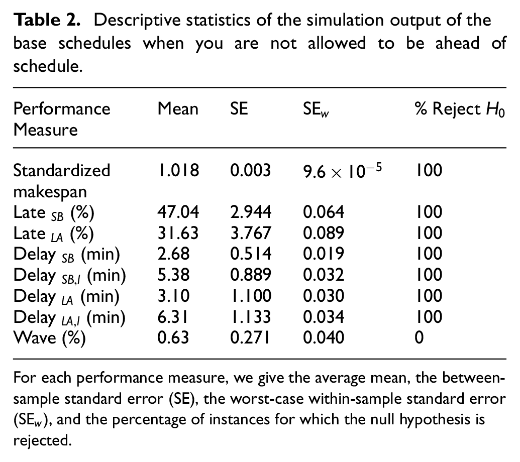
For each performance measure, we give the average mean, the between-sample standard error (SE), the worst-case within-sample standard error ( ${\mathrm{SE}}_w$ ), and the percentage of instances for which the null hypothesis is rejected.

We see that on average, the operation takes 1.8% longer than planned and that for, on average, 47% of the trips, the connector arrives late at the SB. The average delay of these late arrivals is a bit over 5 min. The number of trips for which the connector arrives late at the LA is lower; however, the delay at the LA is approximately 1 min larger than at the SB. This can be caused by the policy that connectors cannot be loaded before the scheduled time at an SB, while it is possible to start unloading at an LA before the scheduled time. Therefore, connectors that arrive earlier at an LA can already unload and depart to the SB and therefore potentially arrive before the scheduled time, which is less likely to occur at LAs. Waves are rarely violated, which is also caused by the inability of connectors to depart before schedule. Therefore, having a significant time difference between two consecutive deliveries is not likely to occur.

In the t-tests, we test whether the realized performance measures differ significantly from the predicted performance measures. In other words, whether the realized makespan is significantly larger than the planned makespan, the percentage of times a connector is late is significant, the delays are significant, and the percentage of waves that are violated is significant. We find that for all instances, the makespan is significantly larger than planned and that connectors incur significant delays. However, the percentage of waves that are violated is not significant. The results show that the buffer time arising in the schedule from the discrete time periods is not sufficient to capture delays when the most optimistic parameters are used to construct the schedule.

We thus find that executing the schedule takes significantly longer than the planned duration. Namely, on average, the realized makespan is 1.8% higher than the planned makespan. However, if connectors would always travel at average speed and have an average (un)loading time, the realized makespan would be on average 2.8% higher. Hence, although the realized makespan is significantly higher, the variability in the speed and (un)loading time results in a better solution compared to when the average speed and (un)loading time are observed.

4.2. The performance of more conservative schedules

To analyze the effect of using more conservative parameters, we determine a schedule using more conservative parameters for the speed of connectors or the (un)loading time using the branch-and-price algorithm of Wagenvoort et al. ⁵ Using a paired t-test, we analyze whether the more conservative parameters have a positive, negative, or insignificant effect on the realized makespan.

Table 3 shows the average simulation output for a given reduction in the speed and increase in the (un)loading time. The percentage of the maximum speed or minimum (un)loading time is given by $p_s$ and $p_t$ , respectively. The corresponding statistical value is given by $v_s$ and $v_t$ , respectively, where “pctl” is used as short for percentile. The average realized makespan is scaled to the planned makespan according to the base schedule constructed using the most optimistic parameters. We see that, generally, the number and value of delays are decreasing as well as the probability that waves are violated. This is not surprising, since connectors are not allowed to be ahead of schedule and more time is scheduled for (un)loading. This allows for capturing delays better.

Table 3.

Descriptive statistics of the simulation output of the schedules using more conservative parameters for the speed ( $s$ ) or (un)loading time ( $t$ ).

$v_s$	$p_s\left(\%\right)$	$v_t$	$p_t\left(\%\right)$	Standardized makespan	${\mathrm{Late}}_{\mathrm{SB}}$	${\mathrm{Late}}_{\mathrm{LA}}$	${\mathrm{Delay}}_{\mathrm{SB}}$	${\mathrm{Delay}}_{\mathrm{SB},l}$	${\mathrm{Delay}}_{\mathrm{LA}}$	${\mathrm{Delay}}_{\mathrm{LA},l}$	Wave
–	100	5 pctl.	101.3	0.994 (0.006)	52.809 (2.407)	60.855 (4.834)	4.828 (0.814)	8.656 (1.106)	10.218 (1.324)	15.739 (0.898)	2.095 (0.895)
–	100	10 pctl.	102.5	0.998 (0.005)	49.260 (2.479)	57.342 (4.784)	3.819 (0.609)	7.233 (0.861)	8.502 (1.058)	13.735 (0.673)	1.960 (0.831)
–	100	15 pctl.	103.8	1.002 (0.005)	45.906 (2.531)	53.510 (4.629)	3.075 (0.421)	6.203 (0.639)	7.098 (0.831)	12.074 (0.467)	1.781 (0.747)
–	100	25 pctl.	106.3	1.014 (0.005)	39.339 (2.55)	44.588 (3.993)	1.881 (0.168)	4.388 (0.341)	4.736 (0.493)	9.252 (0.201)	1.355 (0.555)
–	100	mean	113.2	1.023 (0.005)	42.158 (2.085)	29.900 (2.969)	2.882 (0.376)	6.368 (0.508)	3.015 (0.399)	7.632 (0.315)	1.008 (0.444)
5 pctl.	99.4	–	100	1.019 (0.005)	46.095 (2.943)	28.403 (1.492)	2.217 (0.152)	4.620 (0.308)	2.045 (0.204)	5.230 (0.226)	0.632 (0.271)
10 pctl.	98.7	–	100	1.019 (0.005)	46.095 (2.943)	28.403 (1.492)	2.217 (0.152)	4.620 (0.308)	2.045 (0.204)	5.230 (0.226)	0.632 (0.271)
15 pctl.	98.1	–	100	1.019 (0.005)	46.095 (2.943)	28.403 (1.492)	2.217 (0.152)	4.620 (0.308)	2.045 (0.204)	5.230 (0.226)	0.632 (0.271)
25 pctl.	96.8	–	100	1.019 (0.005)	46.095 (2.943)	28.403 (1.492)	2.217 (0.152)	4.620 (0.308)	2.045 (0.204)	5.230 (0.226)	0.632 (0.271)
mean	93.4	–	100	1.019 (0.005)	46.095 (2.943)	28.403 (1.492)	2.217 (0.152)	4.620 (0.308)	2.045 (0.204)	5.230 (0.226)	0.632 (0.271)

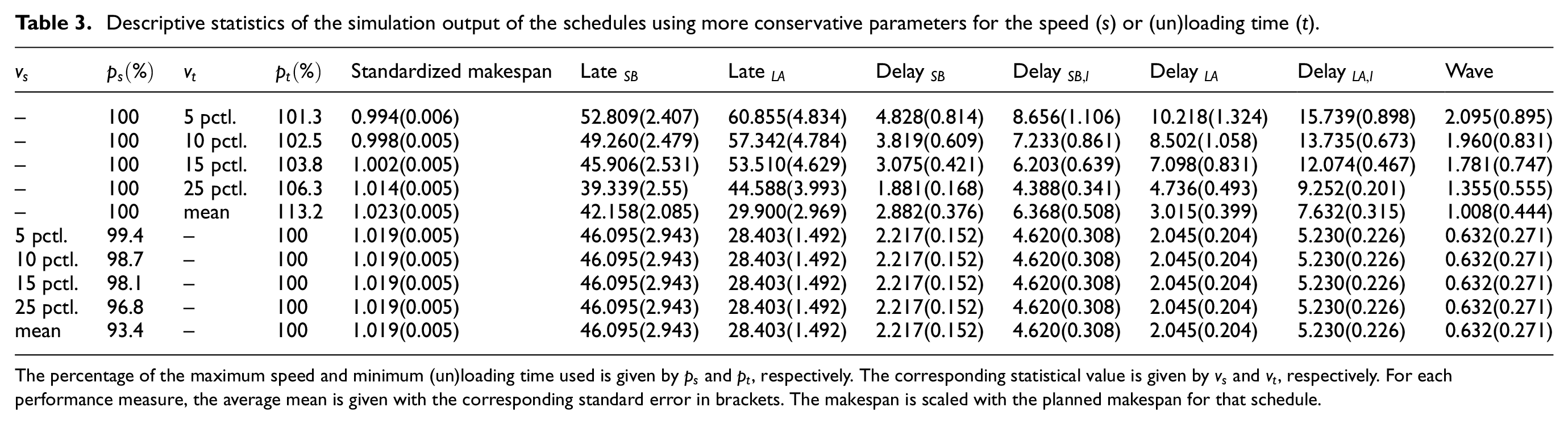
The percentage of the maximum speed and minimum (un)loading time used is given by $p_s$ and $p_t$ , respectively. The corresponding statistical value is given by $v_s$ and $v_t$ , respectively. For each performance measure, the average mean is given with the corresponding standard error in brackets. The makespan is scaled with the planned makespan for that schedule.

Planning more conservatively in terms of the speed results in a realized makespan that is only slightly higher than the average realized makespan for the base schedule given in Table 2. This is likely caused by the fact that there is already some buffer time to capture delays in the basic schedule due to the discretization of the time periods. Using a slightly slower speed can therefore result in the same optimal schedule. For example, if the first 2.5 time periods are required and therefore 3 are scheduled, a slight reduction in the speed used for planning might result in requiring 2.7 time periods, for which still three time periods are scheduled. If this is the case for all connectors, the optimal solution is the same, resulting in an insignificant output of the paired t-test. If the speed reduction does result in requiring an additional time period in order to transport the resources, this has a relatively large effect, as a full extra time period is scheduled for each trip between an SB and LB and/or reverse. For example, if the first 2.9 time periods are required and therefore 3 are scheduled, a slight reduction in the speed can result in requiring 3.1 time periods, and therefore, 4 need to be scheduled when this connector is used, resulting in a different optimal solution.

Since there is no effect of different parameters for the speed in our results, we jointly report them in the remainder of this chapter.

Table 4 gives the results of the paired t-test. Here, for a given percentage of the maximum speed and minimum (un)loading time; Table 4 indicates the percentage of instances a positive, negative, or insignificant change in the realized makespan is observed. We see that being a bit more conservative in the (un)loading time, can have a positive effect on the realized makespan. When the speed is decreased, the realized makespan on all instances is higher or insignificantly different from the realized makespan of the basic schedule. The results thus suggest using a slightly more conservative (un)loading time when constructing a schedule, and therefore, a slightly longer time period length is a more effective way to construct a schedule.

Table 4.

Results of the paired t-test and quantile comparison of the standardized makespan comparing the simulation output of the schedule with more conservative parameters for the speed ( $s$ ) or (un)loading time ( $t$ ) with the output of the base schedule.

				Paired t-test			Quantile comparison
$v_s$	$p_s\left(\%\right)$	$v_t$	$p_t\left(\%\right)$	pos.	neg.	insign.	pos.	neg.	insign.
-	100	5 pctl	101.3	93.33	6.67	0	86.67	6.67	6.67
-	100	10 pctl	102.5	93.33	6.67	0	80.00	13.33	6.67
-	100	15 pctl	103.8	93.33	6.67	0	46.67	20.00	33.33
-	100	25 pctl	106.3	93.33	6.67	0	6.67	93.33	0
-	100	mean	113.2	6.67	93.33	0	6.67	93.33	0
*	*	-	100	0	6.67	93.33	0	6.67	93.33

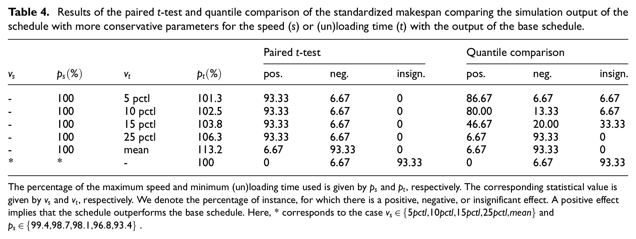
The percentage of the maximum speed and minimum (un)loading time used is given by $p_s$ and $p_t$ , respectively. The corresponding statistical value is given by $v_s$ and $v_t$ , respectively. We denote the percentage of instance, for which there is a positive, negative, or insignificant effect. A positive effect implies that the schedule outperforms the base schedule. Here, * corresponds to the case $v_s\in \{5\mathrm{pctl},10\mathrm{pctl},15\mathrm{pctl},25\mathrm{pctl},\mathrm{mean}\}$ and $p_s\in \{99.4,98.7,98.1,96.8,93.4\}$ .

The negative and insignificant results of the schedules constructed using more conservative speeds are likely caused by the two situations that can occur. Namely, a slight reduction can either result in the same optimal schedule as the number of required time periods to travel between the SBs and LAs remains the same. This gives an insignificant difference in the realized makespan, as the schedules, and hence, the simulation outputs, are identical. Alternatively, a slight reduction can result in scheduling a full additional time period when scheduling a trip from an SB to an LA and/or reverse. This can result in a negative effect on the realized makespan, as connectors are not allowed to be ahead of schedule, and planning a full additional time period can result in a schedule that is too conservative.

Increasing the (un)loading time of the connector affects the schedule in two ways. First, the time scheduled for (un)loading increases, adding more buffer time in the schedule for delays. Second, the time required for a connector to travel between an SB and an LA can either increase or decrease. For example, if initially 15 min time periods are used and it takes 40 min to travel from an SB to an LA, 45 min (three time periods) are scheduled. If the time period length is increased to 20 min, 40 min are scheduled (two time periods), reducing the scheduled time. If, however, the time period length is increased to 17.5 min, 52.5 min are scheduled (three time periods), increasing the scheduled time. Therefore, changing the time period length will always increase the time scheduled for (un)loading but can either increase or decrease the time scheduled for traveling between the locations.

These effects can be seen in Figure 5. Here, we present the distribution of the average realized makespan of the instances for the types of schedules. These show that schedules constructed using a more conservative speed can result in a schedule with a higher makespan and therefore higher realized makespan but are also likely to result in the same schedule and therefore the same realized makespan. When the time period length is adjusted, resulting schedules can be both faster and slower.

Figure 5.

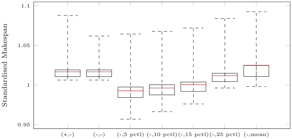
Simulation output for the average realized makespan scaled to the planned makespan of the base schedule. Here, the horizontal axis denotes the types of schedule used of the form ( $v_s$ , $v_t$ ) and * corresponds to the case $v_s\in \{5\mathrm{pctl},10\mathrm{pctl},15\mathrm{pctl},25\mathrm{pctl},\mathrm{mean}\}$ and $p_s\in \{99.4,98.7,98.1,96.8,93.4\}$ .

In practice, a schedule is only executed once and the mean is thus not observed. Therefore, we are also interested in a worst-case performance and we analyze the performance at the 95th percentile. When looking at the quantile comparison, we see that only for the small increases in the time period length, the conservative schedule performs better and that more often the results are insignificant or negative. Hence, the best performance is observed when being only slightly conservative in the (un)loading time for connectors.

4.3. Price of being rigid

The previous results are generated given the policy that a connector is not allowed to be ahead of schedule, which is imposed as preparations are made according to the schedule. This can, however, have a large effect on the realized makespan, as can be seen in Figure 6 which provides an example of an instance that shows the distribution of the realized makespan as a fraction of the planned makespan. The figure shows that being allowed to be ahead of schedule has a positive effect on the expected makespan, but that the effect stagnates the more you are allowed to be ahead of schedule. Namely, the density curve is steep when you are allowed to be no or a limited time ahead of schedule, as there is a high chance you are close to the lowest possible makespan you can attain. However, when you are allowed to be significantly ahead of schedule, the effect stagnates as you are not likely to be significantly ahead of schedule, as can be seen by the scenario $x=60$ . When comparing at the 95th percentile, the performance seems to be similar. Therefore, we analyze the effect of being allowed to be $x$ min ahead of time, for $x\in \{10,30,60\}$ , using a paired t-test and quantile comparison with respect to the scenario in which you are not allowed to be ahead of schedule.

Figure 6.

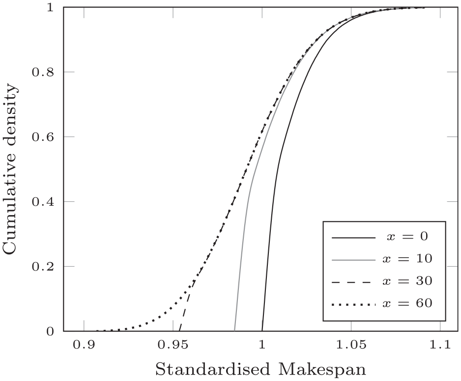
The effect on the distribution of the makespan when you are allowed to be $x$ min ahead of time.

The simulation output when you are allowed to be 10, 30, or 60 min ahead of schedule, can be found in Appendix 2. We highlight some results in Figure 7 regarding the change in the realized makespan and percentage of wave violations for the base schedule. Figure 7(a) shows a decreasing trend in the realized makespan when the minutes you are allowed to be ahead of schedule increase. We see that for some instances, this flexibility does not provide much reduction in the realized makespan, but for others, the makespan can decrease significantly.

Figure 7.

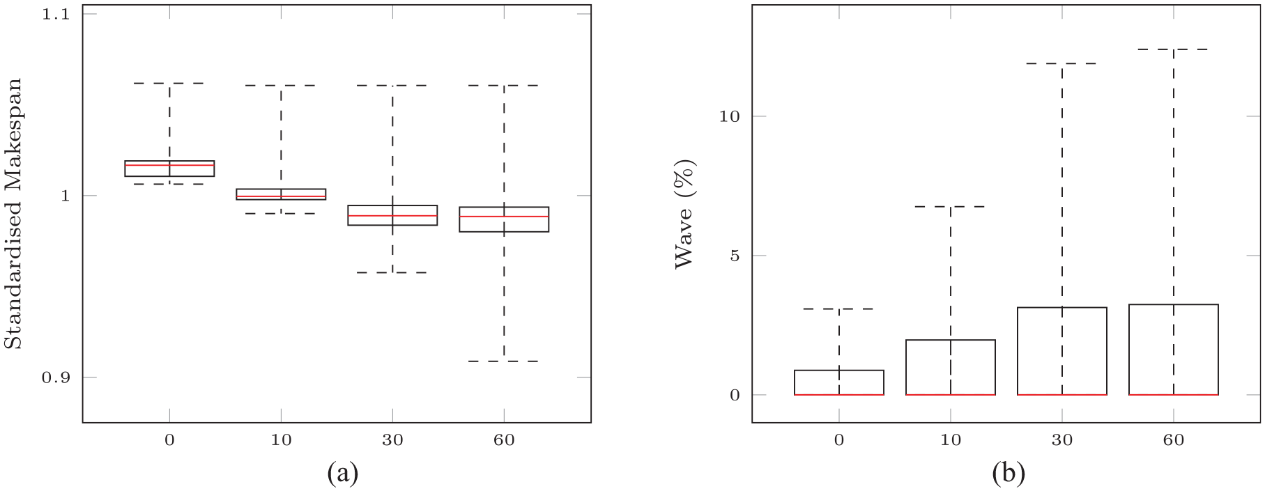
Simulation output for the base schedules when you are allowed to be $x\in \{0,10,30,60\}$ min ahead of schedule: (a) Simulation output for the base schedules for the average realized makespan when you are allowed to be $x\in \{0,10,30,60\}$ min ahead of schedule. (b) Simulation output for the base schedules for the percentage of wave violations when you are allowed to be $x\in \{0,10,30,60\}$ min ahead of schedule.

Figure 7b shows the percentage of wave violations. We see an increasing trend in the wave violations; hence, the more you are allowed to be ahead of schedule, the higher the probability of violating the resource set constraints. This increase comes from the fact that connectors only wait if they know the other connectors joining in the wave will be delayed. If they are still on track, a connector can depart earlier, which can result in a wave violation if the later connectors experience a delay while loading or traveling. When you are allowed to be ahead of schedule, you are thus at a higher risk of violating a resource set constraint. This can result in undesirable and dangerous situations where units that trained together arrive separately from each other and/or the vehicles and other resources they require for their further operation on land. This can result in delays in the operations on land and blockages at the LB.

In the paired t-test, we compare the realized performance measure when you are not allowed to be ahead of schedule with the corresponding realized performance measure when you are allowed to be $x\in \{10,30,60\}$ min ahead of schedule. We find that for all instances, and all schedules, the realized makespan is significantly lower when you are allowed to be ahead of schedule. However, the results from the quantile comparison show that at the 95th percentile, the realized makespans do not differ significantly. Hence, being less rigid will on average ensure the duration of the operation is significantly lower, but in the worst-case, the performance is the same. For the basic schedule, the average realized makespan is 1.8% longer than scheduled (Table 2), which reduces to 0.4%, −0.8%, or −1.3% when you are allowed to be 10, 30, or 60 min ahead of schedule, respectively.

We also find that the percentage of times a connector is late to (un)load reduced significantly when you are allowed to be ahead of schedule. Furthermore, the average delay of connectors is significantly lower as well. However, the average delay, given that you are late, is not always significantly lower. The conditional delays are given in Tables 5 and 6 which show that for some instances the effect on the conditional delay is negative or insignificant.

Table 5.

Results of the paired t-test comparing the simulation output for the conditional delay at an SB ( ${\mathrm{Delay}}_{\mathrm{SB},l}$ ) of the schedule where you are allowed to be $x$ min ahead of schedule with the output of the schedule with $x=0$ .

				$x=10$			$x=30$			$x=60$
$v_s$	$p_s\left(\%\right)$	$v_t$	$p_t\left(\%\right)$	pos.	neg.	insign.	pos.	neg.	insign.	pos.	neg.	insign.
-	100	-	100	80.00	20.00	0	80.00	6.67	13.33	80.00	6.67	13.33
-	100	5 pctl	101.3	46.67	53.33	0	46.67	53.33	0	46.67	53.33	0
-	100	10 pctl	102.5	46.67	53.33	0	46.67	53.33	0	46.67	53.33	0
-	100	15 pctl	103.8	46.67	53.33	0	46.67	53.33	0	46.67	53.33	0
-	100	25 pctl	106.3	46.67	53.33	0	46.67	53.33	0	46.67	53.33	0
-	100	mean	113.2	73.33	20.00	6.67	86.67	0	13.33	86.67	0	13.33
*	*	-	100	80.00	20.00	0	80.00	6.67	13.33	80.00	6.67	13.33

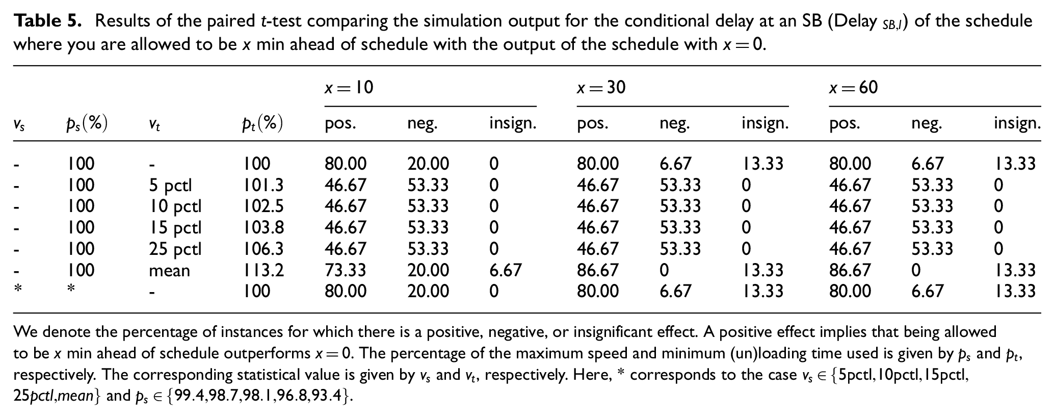
We denote the percentage of instances for which there is a positive, negative, or insignificant effect. A positive effect implies that being allowed to be $x$ min ahead of schedule outperforms $x=0$ . The percentage of the maximum speed and minimum (un)loading time used is given by $p_s$ and $p_t$ , respectively. The corresponding statistical value is given by $v_s$ and $v_t$ , respectively. Here, * corresponds to the case $v_s\in \{5\mathrm{pctl},10\mathrm{pctl},15\mathrm{pctl},25\mathrm{pctl},\mathrm{mean}\}$ and $p_s\in \{99.4,98.7,98.1,96.8,93.4\}$ .

Table 6.

Results of the paired t-test comparing the simulation output for the conditional delay at an LA ( ${\mathrm{Delay}}_{\mathrm{LA},l}$ ) of the schedule where you are allowed to be $x$ minutes ahead of schedule with the output of the schedule with $x=0$ .

				$x=10$			$x=30$			$x=60$
$\mathrm{vs}$	$p_s\left(\%\right)$	$t$	$p_t\left(\%\right)$	pos.	neg.	insign.	pos.	neg.	insign.	pos.	neg.	insign.
-	100	-	100	100	0	0	100	0	0	100	0	0
-	100	5 pctl	101.3	46.67	53.33	0	33.33	66.67	0	33.33	66.67	0
-	100	10 pctl	102.5	66.67	33.33	0	53.33	46.67	0	53.33	46.67	0
-	100	15 pctl	103.8	80.00	20.00	0	80.00	20.00	0	80.00	20.00	0
-	100	25 pctl	106.3	100	0	0	100	0	0	100	0	0
-	100	mean	113.2	100	0	0	100	0	0	100	0	0
*	*	-	100	100	0	0	100	0	0	100	0	0

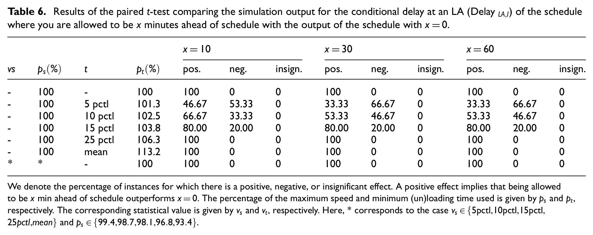
We denote the percentage of instances for which there is a positive, negative, or insignificant effect. A positive effect implies that being allowed to be $x$ min ahead of schedule outperforms $x=0$ . The percentage of the maximum speed and minimum (un)loading time used is given by $p_s$ and $p_t$ , respectively. The corresponding statistical value is given by $v_s$ and $v_t$ , respectively. Here, * corresponds to the case $v_s\in \{5\mathrm{pctl},10\mathrm{pctl},15\mathrm{pctl},25\mathrm{pctl},\mathrm{mean}\}$ and $p_s\in \{99.4,98.7,98.1,96.8,93.4\}$ .

We can identify two types of delays. First, incidental delays, which are delays occurring at one event. For example, a delay during the last trip of a connector, or a small delay upon arrival at a location, due to a longer (un)loading time or travel time, that can be compensated before it arrives at its next location. Second, propagating delays, which are delays that cause delays in the next arrivals too. For example, a connector can have a delay during one of its first trips, which causes subsequent delays as it requires (almost) the full time period to (un)load and/or (almost) the full time periods to travel between the SB and LB.

When a connector is allowed to depart before schedule, the first type of delay is less likely to occur. Namely, a connector can be ahead of time when starting a trip, and therefore still finish on time even though it takes longer to (un)load or travel. However, the second type can still occur, namely, delays at the start can still propagate through the schedule, as the connector did not benefit (much) from being allowed to depart before the schedule time. This can negatively affect the conditional delay.

Table 7 shows the results of the paired t-test on the wave violations. It shows that the results are either insignificant or negative. In the cases where the wave violations do not differ significantly, no wave violations were present. After inspection of these solutions, it appeared that the resource sets were small and either all resources were transported on one large connector, or the wave was small and had high priority such that they were transported immediately at the start of the operation, and hence, they could not experience large enough delays for there to be a violation. In the other cases, we observe a negative effect on the wave violations caused by the higher risk of violating a resource set constraint when you are allowed to be ahead of schedule.

Table 7.

Results of the paired t-test comparing the simulation output for the wave violations of the schedule where you are allowed to be $x$ min ahead of schedule with the output of the schedule with $x=0$ .

				$x=10$			$x=30$			$x=60$
$v_s$	$p_s\left(\%\right)$	$v_t$	$p_t\left(\%\right)$	pos.	neg.	insign.	pos.	neg.	insign.	pos.	neg.	insign.
-	100	-	100	0	33.33	66.67	0	33.33	66.67	0	33.33	66.67
-	100	5 pctl	101.3	0	33.33	66.67	0	33.33	66.67	0	33.33	66.67
-	100	10 pctl	102.5	0	33.33	66.67	0	33.33	66.67	0	33.33	66.67
-	100	15 pctl	103.8	0	33.33	66.67	0	33.33	66.67	0	33.33	66.67
-	100	25 pctl	106.3	0	33.33	66.67	0	33.33	66.67	0	33.33	66.67
-	100	mean	113.2	0	33.33	66.67	0	33.33	66.67	0	33.33	66.67
*	*	-	100	0	33.33	66.67	0	33.33	66.67	0	33.33	66.67

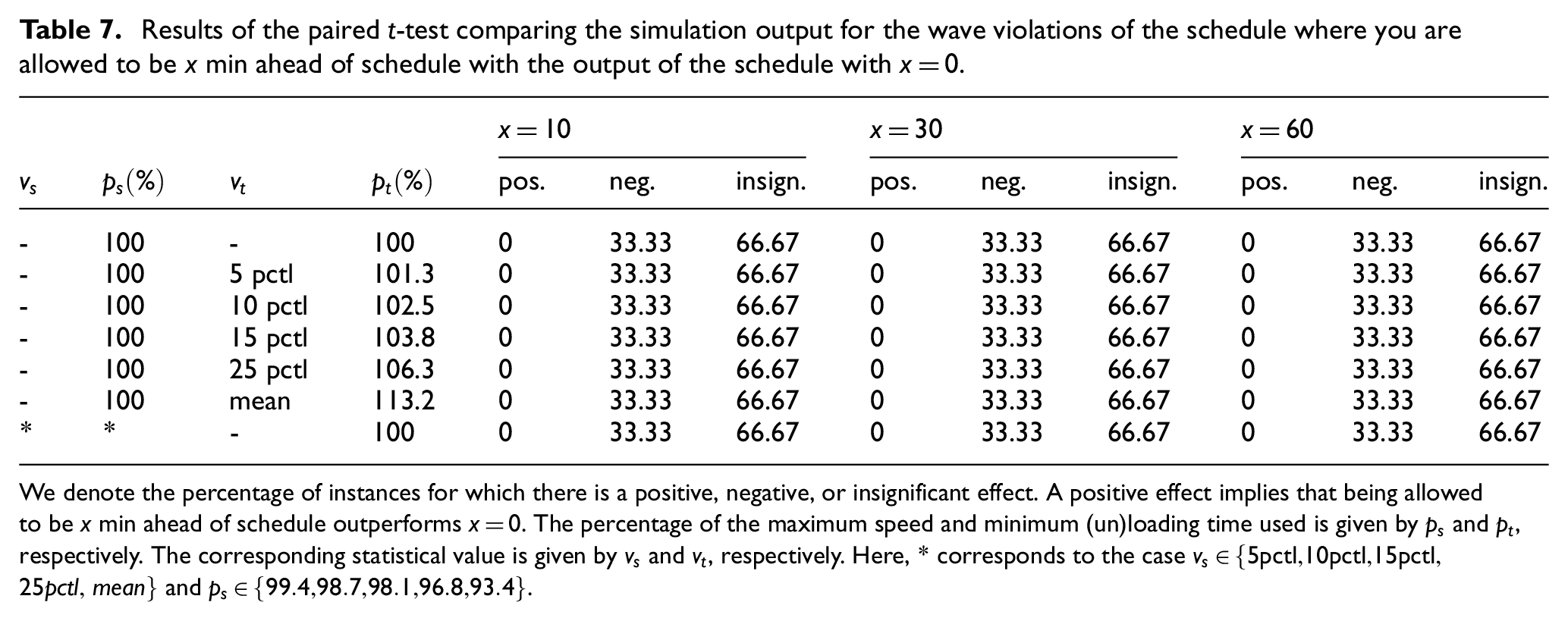
We denote the percentage of instances for which there is a positive, negative, or insignificant effect. A positive effect implies that being allowed to be $x$ min ahead of schedule outperforms $x=0$ . The percentage of the maximum speed and minimum (un)loading time used is given by $p_s$ and $p_t$ , respectively. The corresponding statistical value is given by $v_s$ and $v_t$ , respectively. Here, * corresponds to the case $v_s\in \{5\mathrm{pctl},10\mathrm{pctl},15\mathrm{pctl},25\mathrm{pctl},\mathrm{mean}\}$ and $p_s\in \{99.4,98.7,98.1,96.8,93.4\}$ .

5. Conclusion

In this paper, we developed a discrete-event simulation model that can be used to analyze the performance of a deterministically constructed schedule when these parameters are actually stochastic. This simulation model follows certain policies specifying the order of events and the amount of time connectors are allowed to be ahead of schedule and can be used to evaluate the realized makespan, the percentage of times a connector is late, the average observed delays of connectors, and the percentage of times a resource set constraint is violated. Using such a simulation model can give interesting insights into the effect of using more conservative parameters in the scheduling phase as well as the effect of using different policies in the execution of a schedule. Especially in situations where a schedule is usually only executed once, as in the ship-to-shore problem, a simulation model can be used to gather insights, as new policies cannot be evaluated in experiments.

We use the simulation model to evaluate the performance of a schedule under uncertainty regarding the speed and (un)loading times of connectors as well as the weather conditions. We use a schedule constructed using discrete time periods to analyze whether the room in the schedule is able to capture these delays. Furthermore, we analyze the effect of using more conservative parameters in the construction of a ship-to-shore schedule and the effect of being less rigid in the execution of a schedule, i.e., by allowing connectors to depart earlier than the predicted scheduled time.

Using schedules constructed using a branch-and-price algorithm with discretized time periods, ⁵ we find that the realized makespan is significantly higher (1.8%) when parameters are stochastic; hence, the room in the schedule arising from the usage of discretized time periods does not suffice to compensate for the delay incurred. In more than 30% of the trips, a connector arrives significantly late at the SB or LB. However, the resource set constraints are not significantly often violated.

For the same instances, we generated schedules constructed using the branch-and-price algorithm using more conservative parameters. Here, we either used a more conservative speed or a more conservative (un)loading time. We find that using a more conservative speed does not result in a significantly better performance. In fact, this resulted in either an insignificant or a negative effect on the realized makespan. Using a more conservative speed can result in the exact same schedule due to the discretization of the time periods. When a more conservative (un)loading time is used, we found for most instances a positive significant effect. However, being too conservative can have a counterproductive effect. Since a schedule is not likely to be executed often, the mean performance is never observed. Therefore, we also look at a worst-case performance by evaluating the performance at the 95th percentile. We find that this negative effect of being too conservative can be observed earlier when the worst-case is considered.

One of the simulation policies is that a connector cannot be ahead of schedule. This can have a large effect on the realized makespan, as only negative effects of the stochastic parameters are observed. We therefore consider what happens when the execution of a schedule is less rigid, i.e., a connector is allowed to be a limited time ahead of schedule. Here, we considered 10, 30, and 60 min. This has a positive significant effect on the realized makespan and the percentage of time a connector is late. However, this comes at a risk of violating the resource set constraints.

In practice, if a slight increase in the probability of violating resource set constraints is acceptable, we recommend adopting a less rigid approach in the execution of a schedule. Our findings indicate that allowing departures to be up to 10 min ahead of schedule can lead to significant reductions in the realized makespan. This strategy offers more consistent reduction compared to constructing the schedule using more conservative parameters. However, if minimizing wave violations is a priority, we recommend using more conservative parameters for the (un)loading time in constructing the schedule. Although these showed both positive and negative effects on the realized makespan, we observe only negative and insignificant results when adjusting the speed of the connectors. To limit negative effects, we advise analyzing the buffer time in connector trips before applying more conservative parameters. Furthermore, we advise using only slightly longer (un)loading times to maximize the chance of a smaller expected and worst-case realized makespan.