
Abstract
Modeling and simulation is a proven cost-efficient means for studying the behavioral dynamics of modern systems of systems. Our research is focused on evaluating the ability of neural networks to approximate multivariate, nonlinear, complex-valued functions. In order to evaluate the accuracy and performance of neural network approximations as a function of nonlinearity (NL), it is required to quantify the amount of NL present in the complex-valued function. In this paper, we introduce a metric for quantifying NL in multi-dimensional complex-valued functions. The metric is an extension of a real-valued NL metric into the k-dimensional complex domain. The metric is flexible as it uses discrete input–output data pairs instead of requiring closed-form continuous representations for calculating the NL of a function. The metric is calculated by generating a best-fit, least-squares solution (LSS) linear k-dimensional hyperplane for the function; calculating the L2 norm of the difference between the hyperplane and the function being evaluated; and scaling the result to yield a value between zero and one. The metric is easy to understand, generalizable to multiple dimensions, and has the added benefit that it does not require a closed-form continuous representation of the function being evaluated.
1. Introduction
Modern systems are typically composed of collections of pre-existing subsystems (or components) that are independently developed, optimized, and fabricated for use in multiple applications. The benefits of this “systems of systems” approach are well understood in system design and manufacturing and result in significant cost reductions, improved reliability, and subsystem reuse across multiple systems. It is also true that these benefits extend into the modeling, simulation, and analysis of new systems as the constituent subsystem models have already been developed, refined, and abstracted to provide accurate and efficient system simulations.
Many scientific and engineering models contain functional blocks containing complex-valued signals and functions. For example, antenna design and analysis includes the antenna shape and sub-element arrangement to generate a design based on the associated frequency-domain characteristics which includes the complex amplitude of the desired operating range, nonlinearity (NL) in responses, and other design considerations. 1 Acoustic signal processing is another field where complex-valued signals are important. 2 Ultrasonic imaging can be used to estimate the sea depth by analyzing the echo generated by the rocks or sand on the seabed. Distortions and nonlinearities in the returned signal can be introduced by seabed objects which decrease the quality of a seabed map created using this technology. Hirose et al. proposed a complex-valued-based Markov random field model to visualize the shape of distant boundaries to mitigate these distortions. Adaptive processing of interferometric synthetic aperture radar (InSAR) imaging involves complex-valued electromagnetic-wave signal processing. 3 The InSAR amplitude data correspond to reflectance and the phase to variation in object height. Since the amplitude and phase are inseparable properties of the electromagnetic wave, they are treated as a single complex-valued data entity. In each of these applications, modeling the system requires the use of complex-valued signals and functional blocks.
Modern composite military systems of interest contain functional blocks that are nonlinear. The NL may result from internal states that change over time and apply different logic and mathematical models to signal processing (e.g., detecting signals in noise). For example, there may be some logic using a noise-riding threshold, T, with signals detected as values that are consistently above the noise over some continuous epoch of length tmin > 1, so that noise spikes (t = 1) that are above T are not detected as signals. In this case, the logic imparts discontinuity, and hence NL between the input and output pairs. As the internal state (e.g., of the noise-riding threshold) evolves over time, so does the NL. Systems may also contain signal pre-processing blocks that produce time-invariant transformations of sensor data. The development and use of surrogate approximate models to mimic these transformations enable the study of behaviors over a wider range of input–output values than would be practical using the system itself which may not exist yet, whose models may be restricted or unavailable for use, or when the models may be too computationally expensive for use in system simulation. 4 In these important cases, when a sufficient set of representative input–output pairs can be obtained, it may be possible to use one or more surrogate models to approximate a functional block with sufficient accuracy as defined by the analyst.
Recent progress in the application of artificial intelligence technologies has motivated us to examine the use of machine learning, statistical learning, and neural networks in the surrogate modeling and simulation of systems which process complex-valued signals. Specifically, our current research focuses on investigating the viability of approximating nonlinear complex-valued functional blocks using neural networks. While neural networks are often used to classify and cluster real-world data, they can also be used for function approximation.5,6 Our hypothesis is that the use of neural networks for complex-valued function approximation may reduce computational resource requirements when simulating large systems of systems which process complex-valued signals. Our initial research revealed that the amount of NL contained within a complex-valued function impacts both the accuracy and the amount of computational resources required to approximate the function using a neural network. As a consequence, measuring the degree of NL present in a functional block is essential when approximating the block using neural networks. For this reason, it is necessary to develop a metric to quantify the amount of NL present in time-invariant, complex-valued functional blocks. An NL metric is an essential tool in military modeling and simulation as it enables the analyst to evaluate tradeoffs when using neural networks to approximate complex-valued functions.
In this paper, we introduce a metric for the quantification of NL in multi-dimensional complex-valued functions. The metric is calculated by generating a best-fit, least-squares solution (LSS) linear k-dimensional hyperplane for the function; calculating the L2 norm of the difference between this hyperplane and the function being evaluated; and scaling the result to yield a value between zero and one. The remainder of this paper is organized as follows. Section 2 presents the basic mathematical concepts of quantifying NL in a function of one variable which forms the basis of the proposed metric; section 3 introduces our least squares-based NL metric for k-dimensional complex-valued functions; section 4 demonstrates application of the metric to quantify NL in two complex-valued functional blocks, each of which contains four complex-valued functions; and section 5 provides conclusions and future research directions.
2. Quantification of NL of a function of one variable
A linear equation is one in which the outputs have a constant, multiplicative proportional relationship to the inputs. Conversely, a nonlinear equation is one in which the outputs cannot be simply related to the inputs by such a constant of proportionality. In engineering and the sciences, nonlinear systems are of great interest, as most real physical systems exhibit nonlinear behaviors.
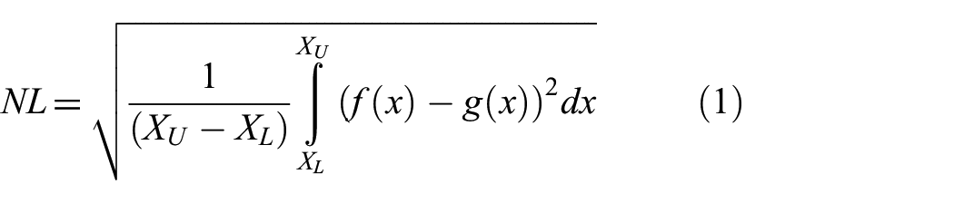
The concept of a linear function of one variable is simple to visualize and is relatively easy to identify by inspection of a plot of a function’s input/output relationship. If we think of quantifiable NL as being the measure of divergence of a nonlinear function from a straight line over some domain, we can develop an associated metric which quantifies this divergence. Existing work has proposed a quantifiable measure of NL in the real domain.7–9 Emancipator and Kroll 9 discuss the need for a quantitative measure of NL in the real domain. They define a “(dimensional) nonlinearity” method as the square root of the mean of the square of the deviation of the response curve from a straight line, where the straight line is chosen to minimize the NL. Furthermore, they propose that the NL metric should be some measure of the average deviation of a response function from a “best-fit” straight line over the interval of interest. This paper extends previous works to provide an alternative nonlinear metric approach in the more general case that includes complex-valued functions. The method of defining a function’s NL in terms of deviation from a linear function is useful even in multi-dimensional real and complex spaces where visualization becomes impractical.
2.1. Quantification of NL of a real function of one variable
For example, consider the periodic function
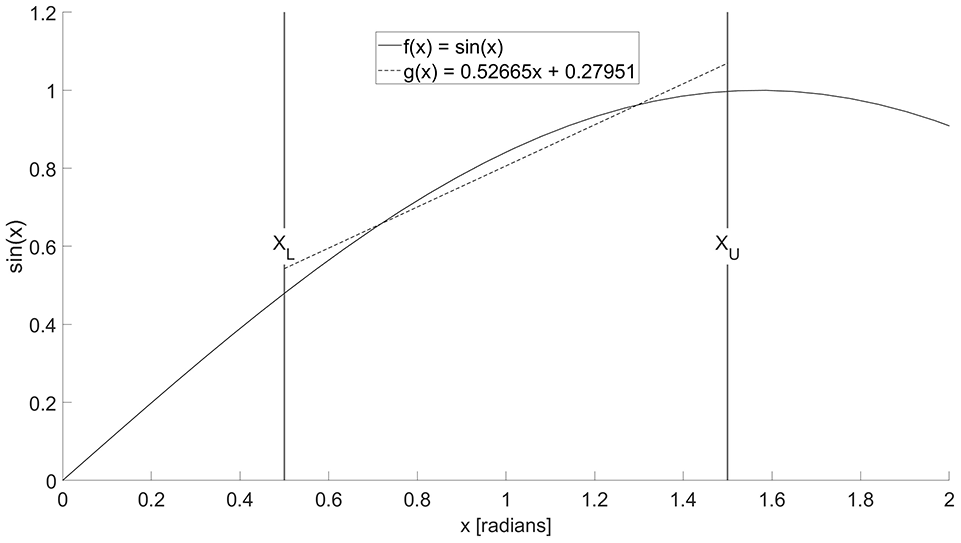
Plot of a nonlinear function
Determining the best-fit line
This approach is tractable when
2.2. Quantification of NL of a complex function of one variable
A complex number is an element of a number system that contains both real and imaginary components. Every complex number can be expressed in the rectangular coordinate form
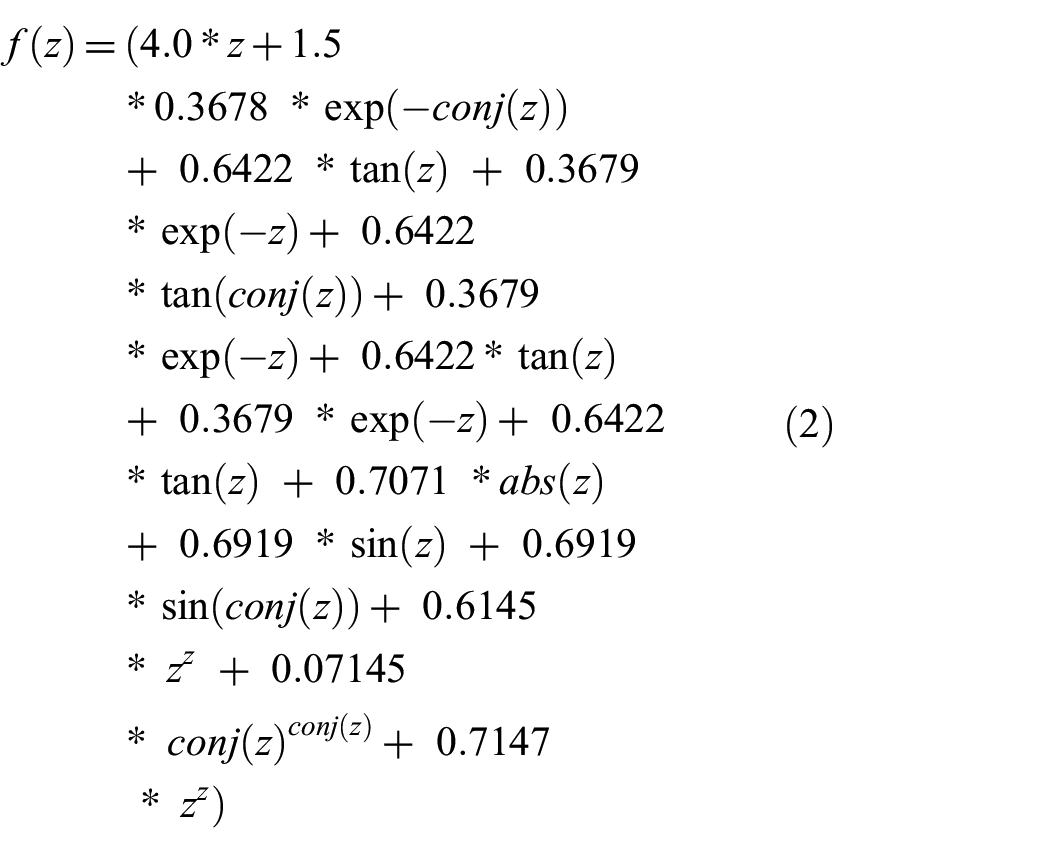
Consider the MATLAB code for an arbitrary complex-valued function
We can express the domain of a complex number
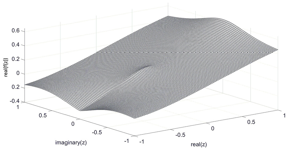
Surface plot of the real part of the nonlinear complex-valued function
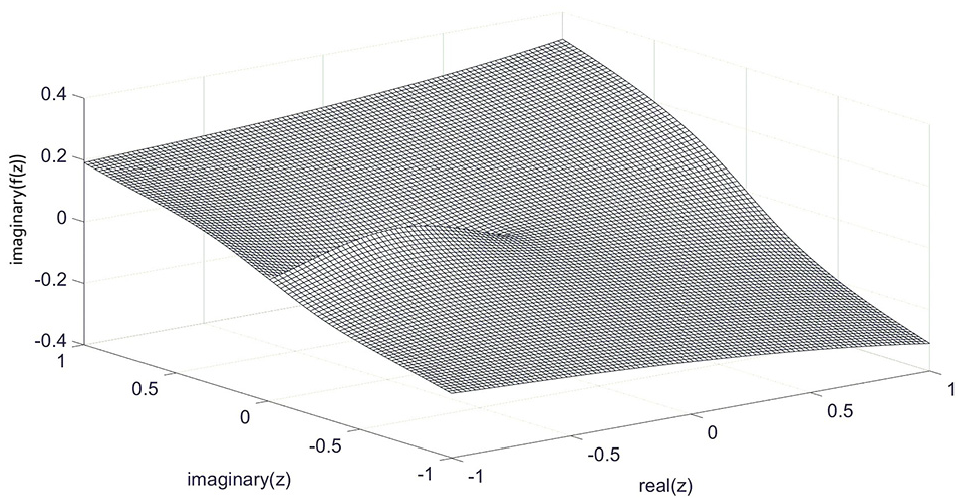
Surface plot of the imaginary part of the nonlinear complex-valued function
Determining the associated integrals of the underlying function from measured data, in this case, is impractical when compared to the case of a function with one real variable as discussed in Emancipator and Kroll.
9
One possible method for finding estimates for the required integrals could be to use an approximation of the true response function
3. Quantification of NL in k-dimensional complex-valued functions
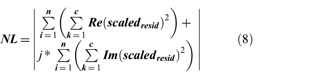
Since the area of interest here is modeling of functions with more than one complex argument, we define an NL metric that is calculated as the absolute value of the sum of squared error between the best-fit k-dimensional hyperplane (where k is the number of arguments) and a discrete set of input–output “ground truth” data. The use of discrete data points eliminates the need to obtain the continuous functional representation. “Best-fit” in this case is determined by finding the hyperplane that minimizes the sum of the squared differences between the true values and the associated points on the hyperplane.
For example, in the three-dimensional case (k = 3), the general equation for a plane

where the
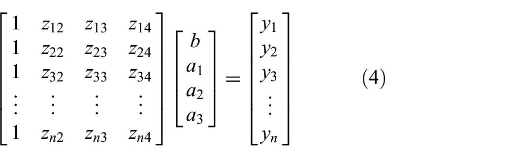
where the number of rows,

When we solve for the plane parameters
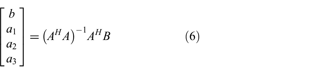
After solving for the parameters, Equation (6) is used to construct the best-fit k-dimensional linear hyperplane. Since we want to ensure the NL metric is unaffected by constant relative change, we first divide the residuals by the range of the true output values as shown in Equation (7):

where
where

In the case where the relationship between the input and output is linear, the LSS provides an approximation that deviates from the true solution on the order of the IEEE 754 machine epsilon precision standard (~10−30).
12
This approach is valid for both the real and complex domains as shown by Elgot.
11
Furthermore, as the input/output relationship becomes increasingly nonlinear, the accuracy of the LSS drops off proportional to the number of observations (n). In the complex domain, this can be seen by observation of the NL calculation
As a straightforward example, we can apply this method to
Note that

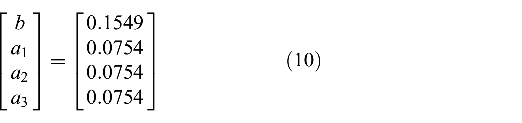
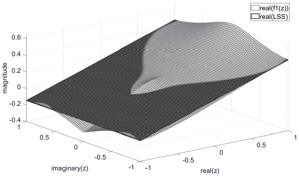
We can now create plots which help visualize the foundation of the NL metric. Figure 4 shows the surface plot for the real part of
Surface plot of the real part of the nonlinear complex-valued function
Surface plot of the imaginary part of the nonlinear complex-valued function
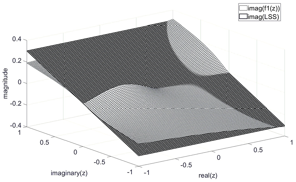
The differences in the functional response between best-fit LSS hyperplane and the actual function response for the real part (Figure 4) and the imaginary part (Figure 5) are the basis for the NL metric shown in Equation (8). A surface plot of the calculated differences between best-fit LSS hyperplane and the function response for the real and imaginary parts is illustrated in Figures 6 and 7, respectively.
Surface plot of the differences between best-fit LSS hyperplane and the actual function response for the real part.
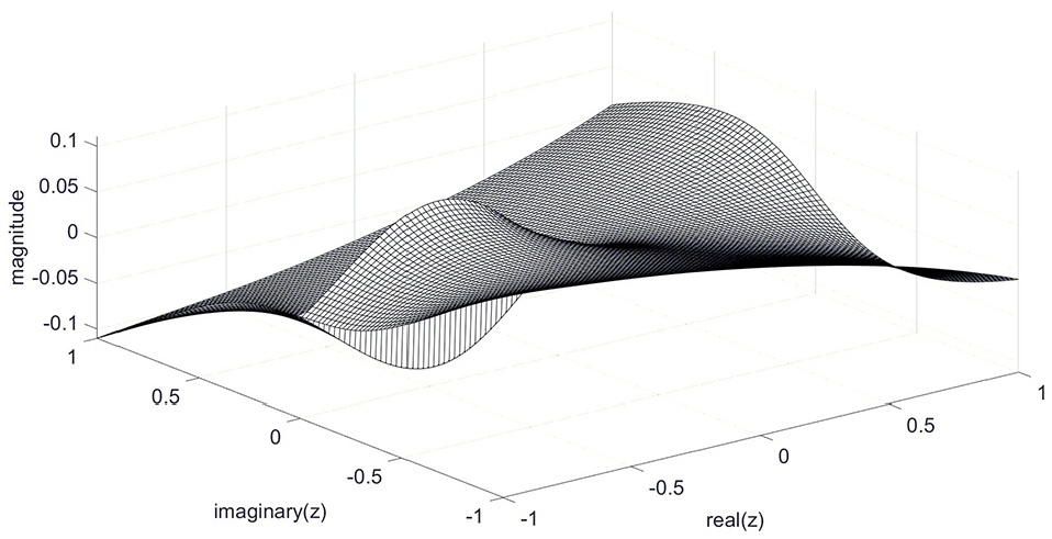
Surface plot of the differences between best-fit LSS hyperplane and the actual function response for the imaginary part.
Using actual values for
In some cases, it may be desirable to provide an NL measure of a complete functional block containing multiple inputs and outputs. In this case, visualization of the method becomes problematic; however, the underlying principles still hold. Assuming we have
4. Application of NL quantification to complex-valued functional blocks
In this section, we demonstrate the use of the NL metric to quantify the NL in complex-valued functional blocks.
4.1. A functional block
In general, a functional block contains multiple functions of multiple variables. Consider, e.g., a four-input, four-output functional block as shown in Figure 8. In this case, we have four independent complex-valued inputs,
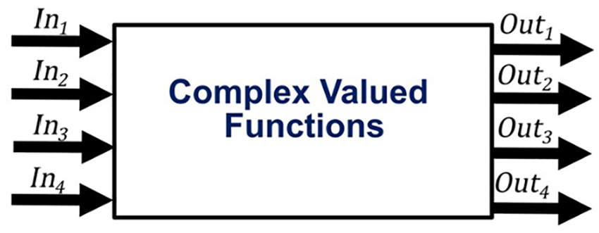
Block diagram of the input/output relationships for a four-input, four-output complex-valued functional block.
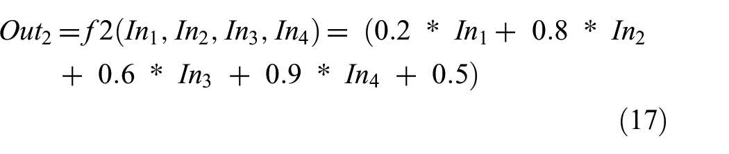
Each of the four outputs is an independent function of four-input variables as shown in Equations (12)–(15) as follows:


4.2. Input and output data
In the two examples that follow, four independent input vectors of 1000 complex elements were generated from a truncated random normal distribution in the real interval
Input data pulled from a truncated random normal distribution from the interval
The application of the input data to the functional block yields a
4.3. Example 1: a linear four-input, four-output complex-valued functional block
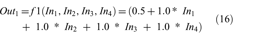
In our first example, we present a four-input, four-output functional block that only contains linear operations as shown in Equations (16) through (19) as follows:
Calculating
Calculated hyperplane parameters for approximating
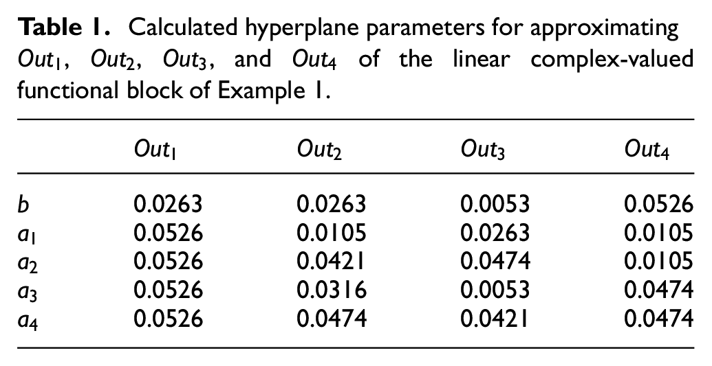
These parameters allow the construction of the linear hyperplane that best-fits the function for each output
Calculated
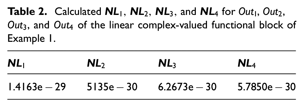
Now showing the associated values using the
Calculated
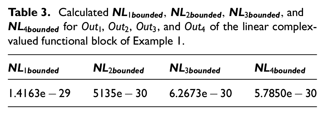
The individual NL values give insight to which outputs contribute the most to the overall NL. In this case,
Figure 10 shows a scatter plot of the resulting complex-valued true responses labeled on the plot as “Data” with circles and the “LSS approximation” labeled with asterisks plotted with the real and imaginary values on the x- and y-axes, respectively. The plot illustrates the high level of accuracy of the calculated linear hyperplane using the LSS approach when the underlying multi-variable complex functions are linear.
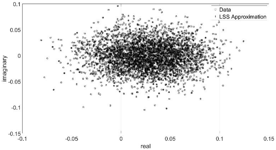
Plot of output from the linear complex-valued multi-variable function with the imaginary component of the output on the y-axis and the real component on the x-axis.
4.4. Example 2: a nonlinear four-input, four-output complex-valued functional block
In our second example, we present a four-input, four-output functional block that contains nonlinear operations. Nonlinear, time-invariant signal pre-processing blocks often multiply complex input signals by trigonometric functions (e.g., sin for frequency translation), exponential functions (e.g., Fourier transforms for generating image features), absolute value functions (e.g., as precursors to the application of logic in subsequent blocks), and other related nonlinear transformations. Without loss of generality, Equations (20)–(23) generate an illustrative four-input, four-output block represented in the format used in the MATLAB software package to generate the functions and data developed in this example:
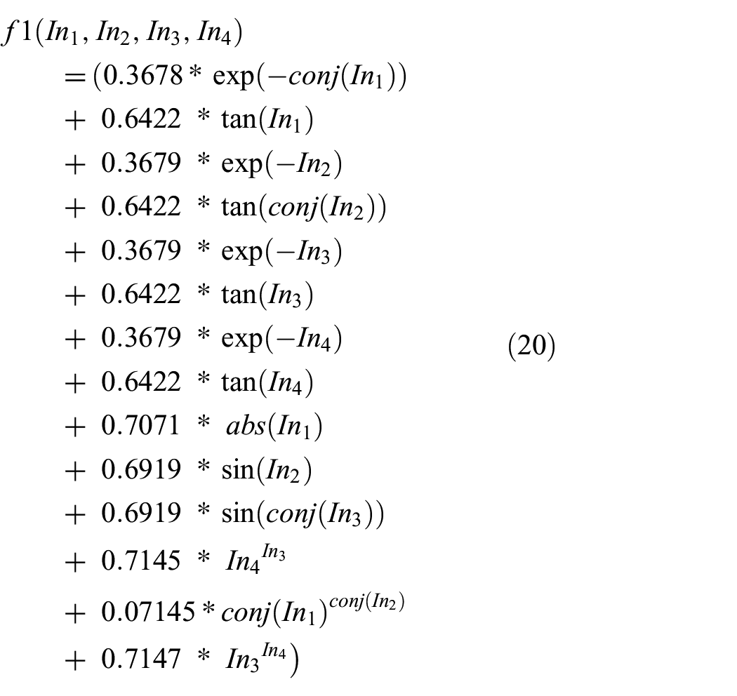
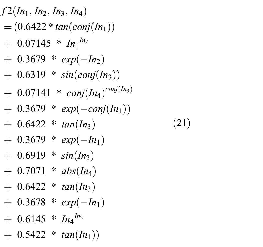
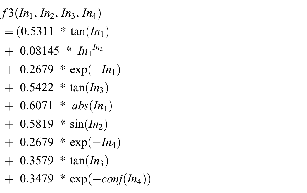
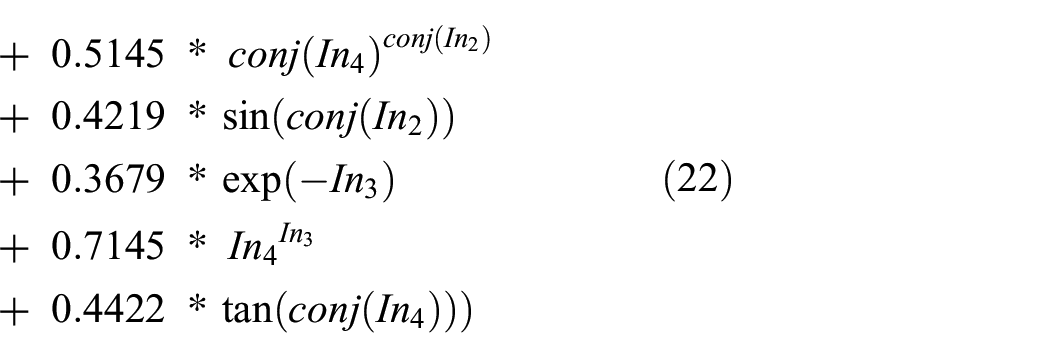
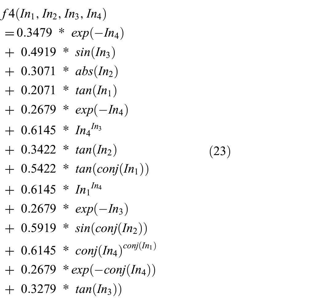
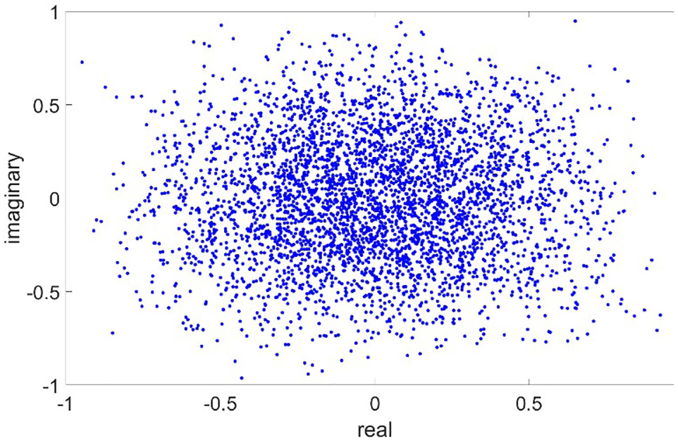
Figure 11 shows a scatter plot of the complex-valued responses plotted with the real and imaginary values of the input on the x- and y-axes. By visual inspection, it can be seen that the LSS approximation is far less accurate in this nonlinear complex-valued function scenario. This is just as we saw in Figure 1 where the linear approximation of a nonlinear function is not a good predictor of the function.
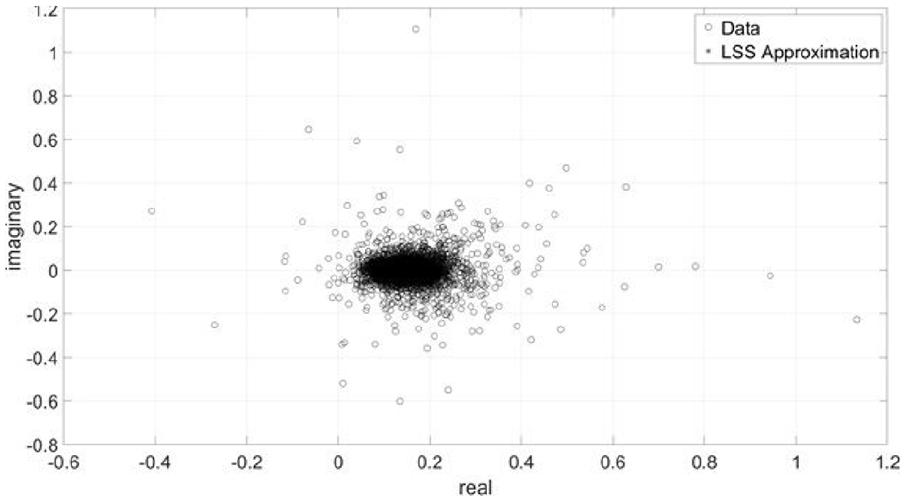
Plot of output from the nonlinear complex-valued multi-variable function with the imaginary component of the output on the y-axis and the real component on the x-axis. Notice that the plot shows that the LSS approximation is not a good predictor of the actual function.
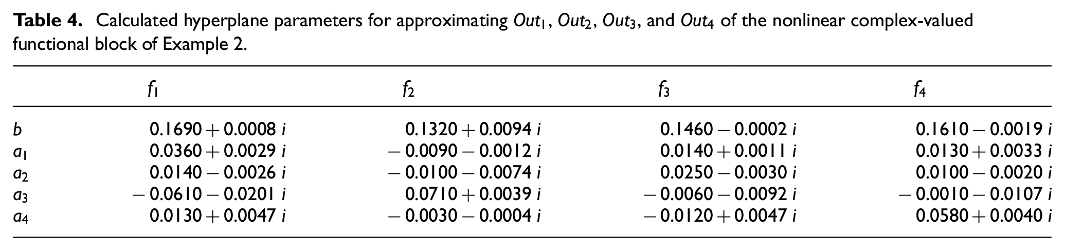
The parameters shown in Table 4 allow the calculation of the approximations for
Calculated hyperplane parameters for approximating
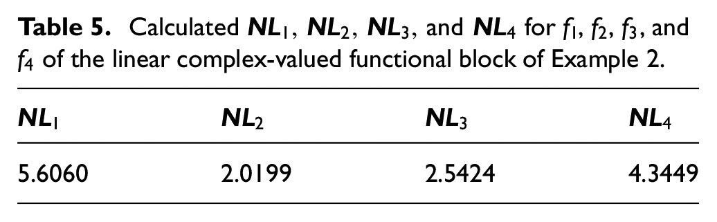
Calculated
Or using the bounded
Calculated
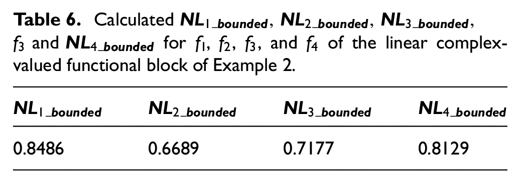
The individual NL values give insight to which functions contribute the most to the overall NL. In this case,
In addition, since the least-squares technique is highly sensitive to outliers, or data points that do not follow the pattern of the other observations, these types of data points will disproportionately influence the NL metric. The outcome will be indication of a more nonlinear function than would be inferred if the offending outliers were not present. This is not typically a problem if the input data are drawn from a normal distribution from the interval discussed previously and the underlying true complex-valued nonlinear behavior is not ill-conditioned. 13 Although real-world systems cannot constrain their inputs to be drawn from a well-behaved normal distribution, the input distribution generates the NL metrics that provide significant insight into the degree of NL present in the block being modeled.
5. Conclusion and future work
In this paper, we introduced a metric for quantifying NL in multi-dimensional complex-valued functions. The metric is based upon existing NL metrics developed for the real domain and is extended to quantify NL in k-dimensional complex-valued functions. The metric is easy to understand, generalizable to multiple dimensions, is invariant to linear scaling, and does not require a closed-form continuous representation of the function being evaluated.
Using the knowledge and experience gained through this work, our research is focused upon evaluating the strengths and weaknesses of various nonlinear complex-valued function approximation techniques. Specifically, we are focused upon understanding the tradeoffs in accuracy, performance, and resource utilization when approximating complex-valued, nonlinear functions using complex-valued neural networks. Future work will explore these tradeoffs, as a function of NL, when generating surrogate models to approximate complex-valued functional blocks. It is expected these results will inform others who are seeking to use neural network-based surrogate models. Ideally, the use of our metric to quantify NL in complex-valued functional blocks will provide researchers a means to predict the required neural network architecture, model parameters, and resources necessary to accurately surrogate model a complex-valued functional block as a function of its NL.
Footnotes
Disclaimer
The views expressed in this paper are those of the authors and do not reflect the official policy or position of the US Air Force, the Department of Defense, or the US Government.
Funding
The author(s) disclosed receipt of the following financial support for the research, authorship, and/or publication of this article: This work was supported by the Laboratory for Telecommunication Sciences (grant number 5703400-000-2121)