
Abstract
The purpose of this work is to analyze the heat transfer characteristics of Vascomax®C300 during high-speed sliding. This work extends previous research that is intended to help predict the wear-rate of connecting shoes for a hypersonic rail system at Holloman Air Force Base to prevent critical failure of the system. Solutions were generated using finite element analysis and spectral methods. The frictional heat generated by the pin-on-disk is assumed to flow uniformly and normal to the face of the pin and the pin is assumed to be a perfect cylinder resulting in two-dimensional heat flow. Displacement data obtained from the experiment is used to define the moving boundary. The distribution of temperature resulting from transient finite element analysis is used to justify a one-dimensional model. Spectral methods are then employed to calculate the spatial derivatives improving the approximation of the function which represents the data. It is concluded that a one-dimensional approach with constant heat transfer parameters sufficiently models the high-speed pin-on-disk experiment.
1. The pin-on-disk experiment
The pin-on-disk experimentation configuration, seen in Figure 1, was set up and conducted by the Air Force Research Laboratory at Wright-Patterson Air Force Base. The pin has a radius of 0.00635 meters and protrudes a length of twice the radius past the clamp as seen in Figures 1 and 2. Displacement was captured by a LDI-119 linear variable inductive transducer position sensor. Force was measured using a LC501 steel cantilever beam. Force and displacement were recorded every
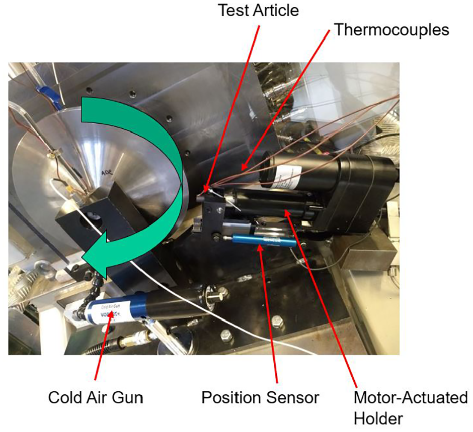
Pin-on-disk experiment configuration.
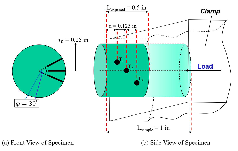
Pin schematic.
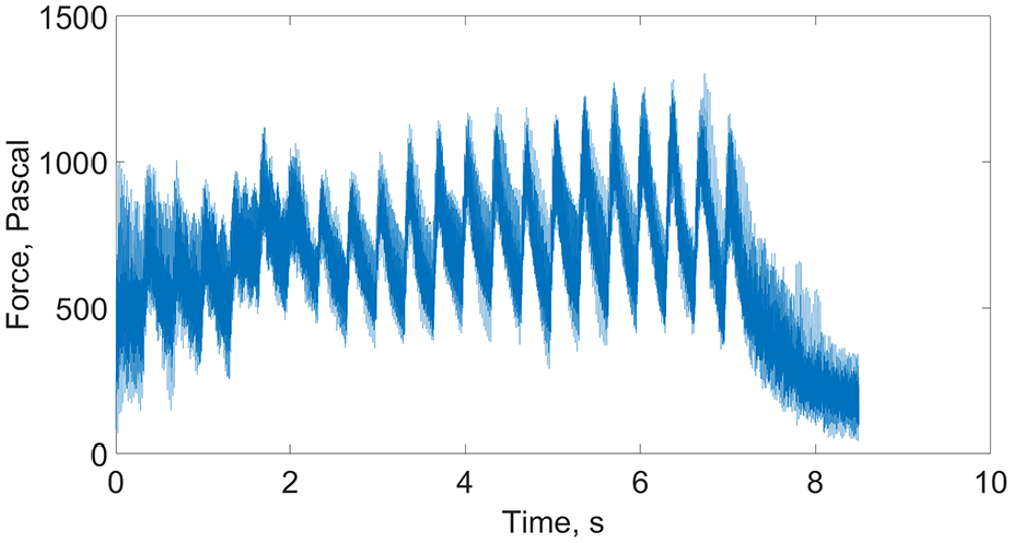
Raw force data.
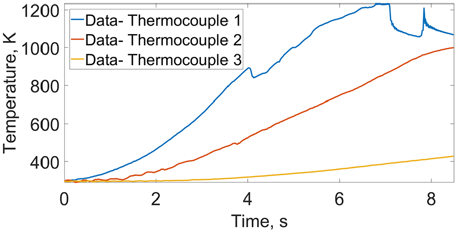
Raw thermocouple temperature data.
The raw data from the experiment exhibits noise and irregularities. The force was maintained manually pressing on the end of the cantilever beam. While the technician did their best to maintain a constant pressure on the pin, it is clear that vibration effects of the friction and the manual adjustments generated considerable noise to the forcing data as seen in Figure 3. The thermocouple closest to the disk (thermocouple 1) has an irregularity at 4 seconds that is unexplained. After 5.5 seconds, this thermocouple begins to read temperatures that exceed the rated threshold. Therefore, the data for thermocouple 1 cannot be trusted to be within the error tolerance after 5.5 seconds. At 7 seconds, there is an irregularity due to a drop in force and faulty readings by the thermocouple. The displacement, shown in Figure 5 is the smoothest, most regular, raw data. The smoothness of the data indicates that vibration effects did not play a large role in the collection of displacement data as it did in the forcing data. However, note in Figure 1 that the position sensor is not located in-line with the pin so that there may have been some loss of information through the connecting system.
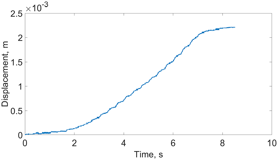
Raw displacement data.
2. Prologue
In 2008, a special run of the HHSTT was conducted. The sled system was highly instrumented to record measurements regarding the extreme aerodynamic forces the sled system undergoes. Previous work1,2 used the 2008 test data as a baseline for the models in their research. Alban utilized a two-dimensional Finite Elements Analysis (FEA) model for the connecting shoe. Alban’s model predicted melt temperatures would be reached inside of the shoe (away from the leading edge). Alban et al. 1 suggests that this would result in additional material wear that the model was not capable of removing. DeLeon looked to improve upon the wear removal modeling and abandoned the FEA approach, focusing instead on a one-dimensional Finite Difference Method (FDM) model. DeLeon et al. 2 improved Alban’s model by considering material removal from the surface through the thickness of the shoe instead of only at the surface.
In 2019, a different approach was taken by conducting a pin-on-disk experiment to generate data for the research. 3 While the pin-on-disk experiment does not reach nearly the same velocity profiles as the sled system, data collection and modeling processes are greatly simplified. Traditional pin-on-disk experiments, such as performed by Ashby and Abulawi, 4 are conducted with velocities on the order of 1 to 10 meters per second. The pin-on-disk design used by Boardman et al. 3 has capability of reaching over 40 times that of the traditional test velocity, but experiments were conducted at a maximum of 240 meters per second.
This work continues the research using the data obtained by the pin-on-disk experiment. Two separate numerical solutions will be generated and discussed for the non-linear heat equation with a moving boundary. Data from the high-speed pin-on-disk experiment is used to compare each model to observation. Finite element analysis and spectral methods each provide unique approximations of, and insight to, the progression of, heat transfer through the pin. FEA will be used to show that a steady-state solution cannot effectively represent the data, leading to transient solution methods. Finite element analysis had not been previously applied to this particular pin-on-disk experimental setup, although finite elements had previously been applied to model slipper wear during a run of the hypersonic rail car.
1
Transient FEA in two-dimensions shows convection negligibly contributes to the solution, effectively reducing the model to one-dimension. Using constant thermal properties, the transient finite element is shown to qualitatively represent the thermocouple data well. Investigation into whether variable parameters can provide a better model is performed with spectral methods. Using variable definitions for the parameters in the thermal diffusivity relation (
3. Assumptions concerning the tribology of the system
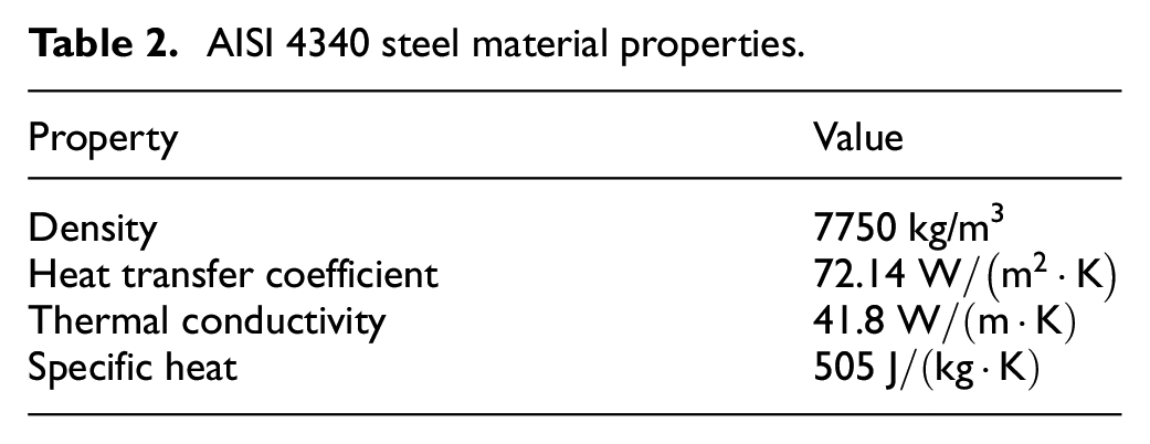
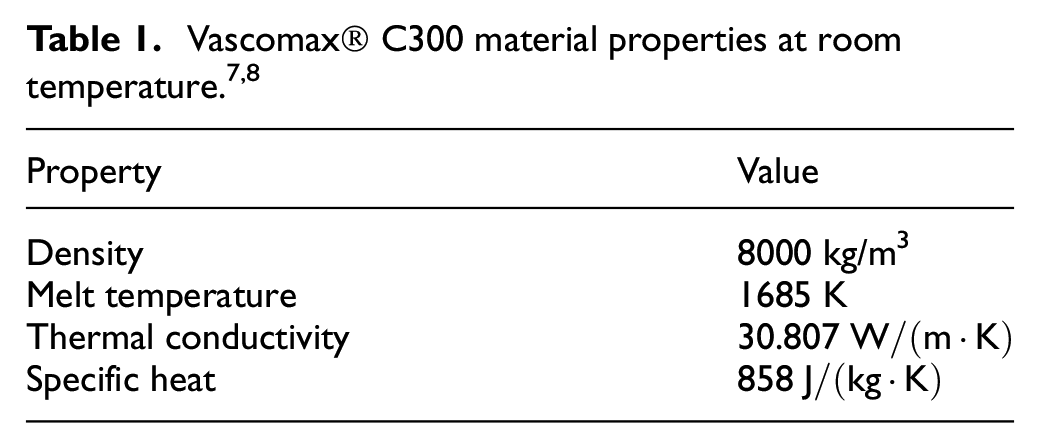
Tribology is the study of the interaction between surfaces in contact. Friction refers to the force that resists sliding. Despite having been studied since prehistoric times, friction has not received a full physical explanation, but there are two basic issues at play: the nature of the friction force and the energy dissipation mechanism. 5 In other words, we look to understand how much heat will enter the system due to friction, and how that heat will conduct through the system. Tables 2 and 3 provide a summary of thermal properties of the pin (Vascomax® C300) and the disk (AISI 4340) that are used in this study.
AISI 4340 steel material properties.
Finite elements analysis material removal.
Flux density,

The Partition Function,
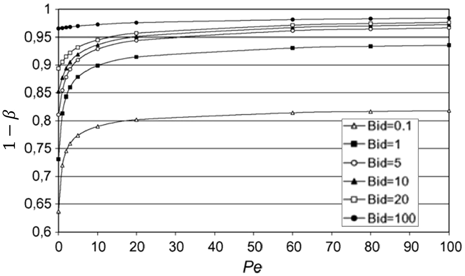
Laraqi partition function.
The coefficient of friction,

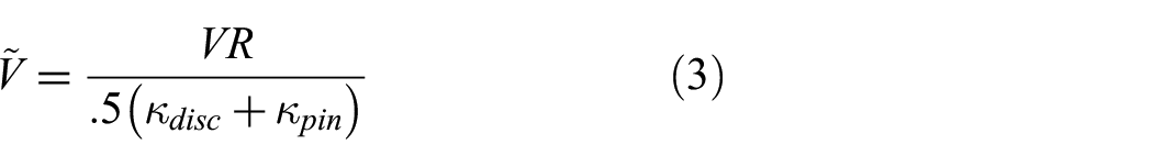
Thermal diffusivity,
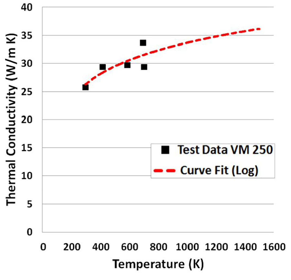
Thermal conductivity of Vascomax® 250.
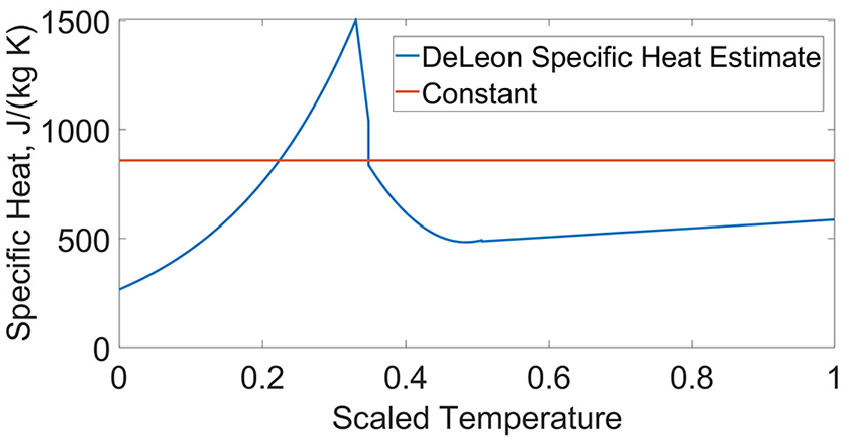
Specific heat approximations of Vascomax® 300.
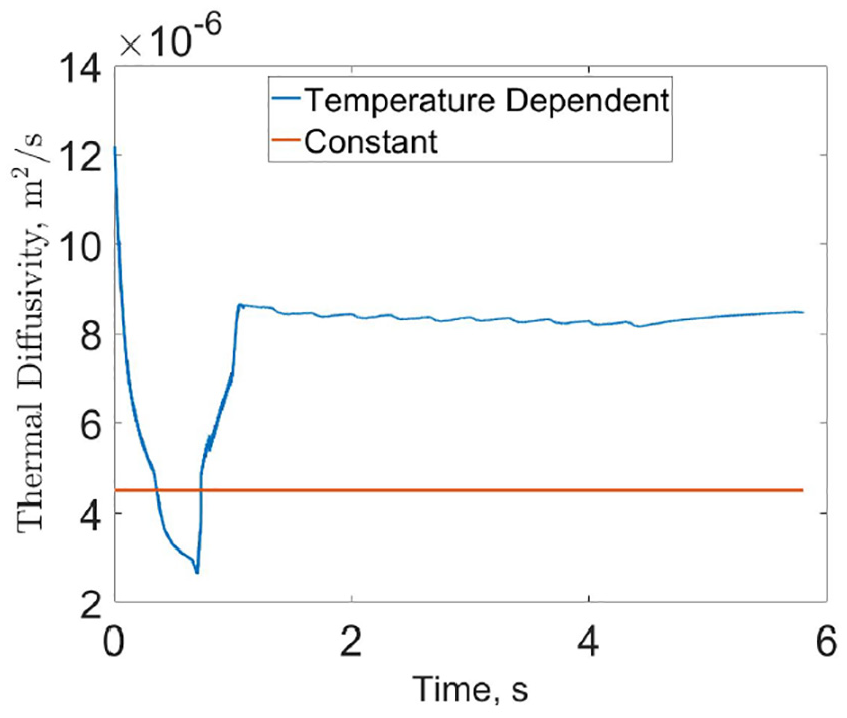
Thermal diffusivity approximations of Vascomax® 300.
The clamp is assumed to be a heat sink that maintains ambient temperature. We use the same convection coefficient for the surrounding air as was previously assumed to be 25
4. Finite element analysis
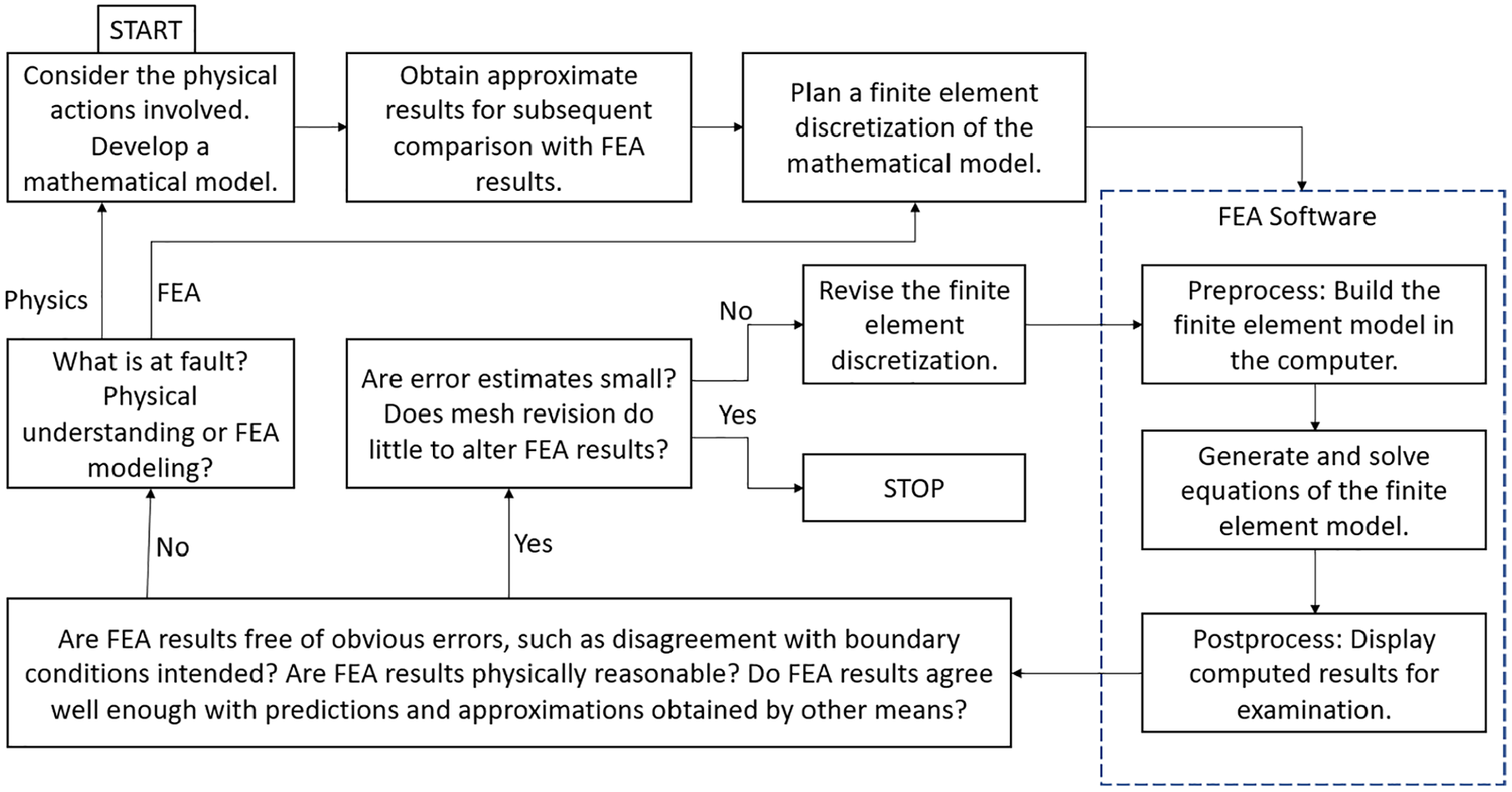
While developing the FEA model the flowchart in Figure 10 was followed. 9 First, a mathematical model was developed and the empirical data were obtained for subsequent comparison to the FEA results. The model was then built using FEA software 10 with initial discretization chosen based upon the thermocouple and displacement locations. We use the displacement data at 1 second intervals to define a non-linear problem with a moving boundary for the FEA by moving the flux boundary inward and removing the elements to model the material being worn away. Several outputs are displayed for examination after solutions were found. The mesh was refined until the refinement no longer significantly altered the results.
FEA flowchart.
The assumption of uniform heat flux across the face of the pin is sufficient to reduce the pin model to two dimensions. As a result, every plane which is normal to the pin face and cuts through the center of the pin face, as shown in Figure 11, will have the same temperature profile. As a result, the pin-on-disk can be viewed as a two-dimensional plane heat transfer problem. Redrawing the pin from Figure 2 under all the assumptions produces the schematic shown as the two-dimensional plane object in Figure 12 where the three thermocouples have been projected onto the same plane.
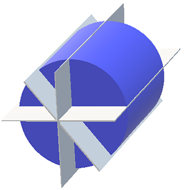
Planes through the center, and normal to, the face of a cylinder.
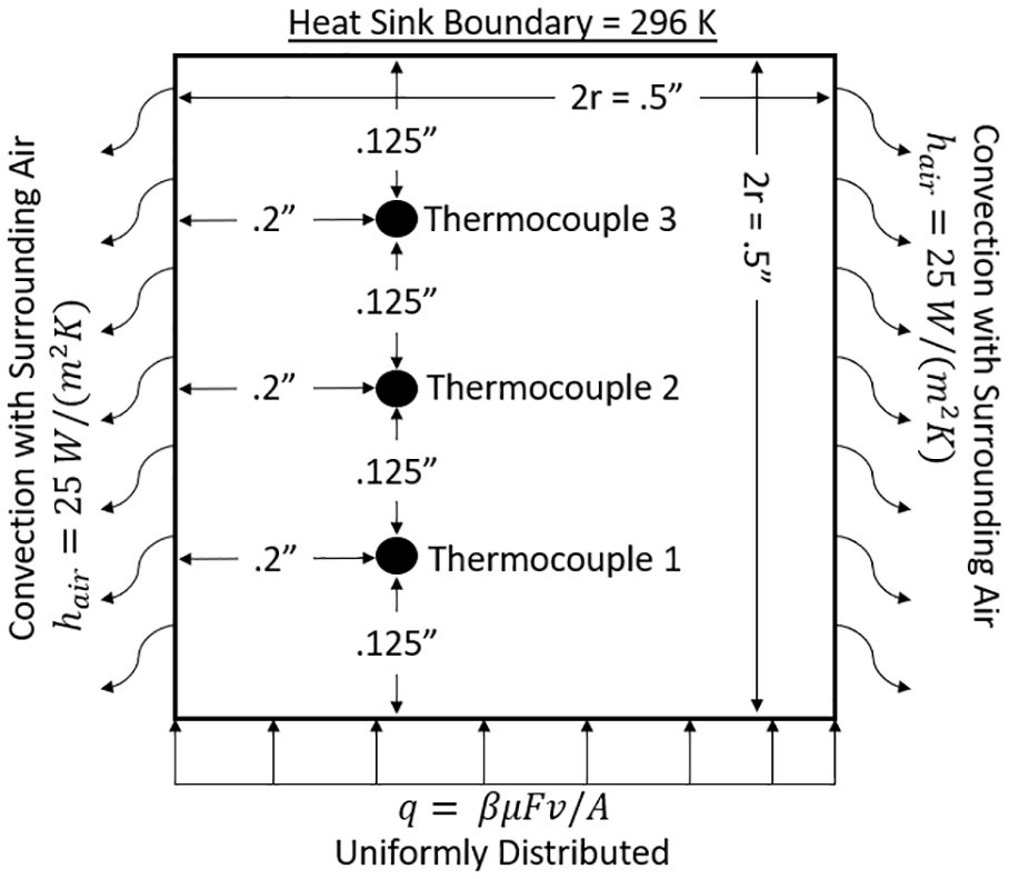
Plane model of the pin.
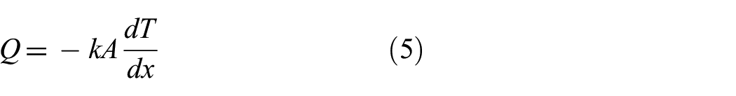
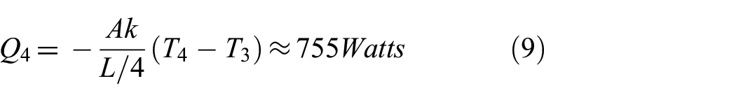
In order to double check that the model has been correctly set up in the software, and in order to properly serve the first three boxes of our flowchart, a one-dimensional steady-state model was considered and compared against the computer model. Starting from conservation of energy the basic finite elements matrix equation is given in Equation (4). 11 The heat rate (heat flow per unit time) is given in Equation (5). 11

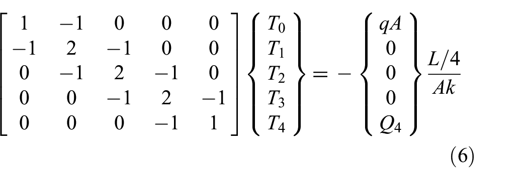
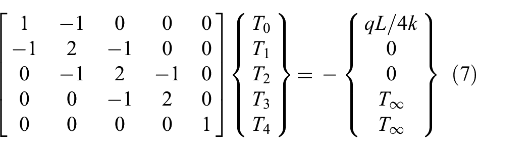
Reducing Figure 12 to 1d and solved the steady-state problem using four elements the problem would reduce to Equation (6) containing five nodes. Assuming that the lengths of the elements are equal, so that the interior nodes represent the three thermocouples; constant thermal conductivity;
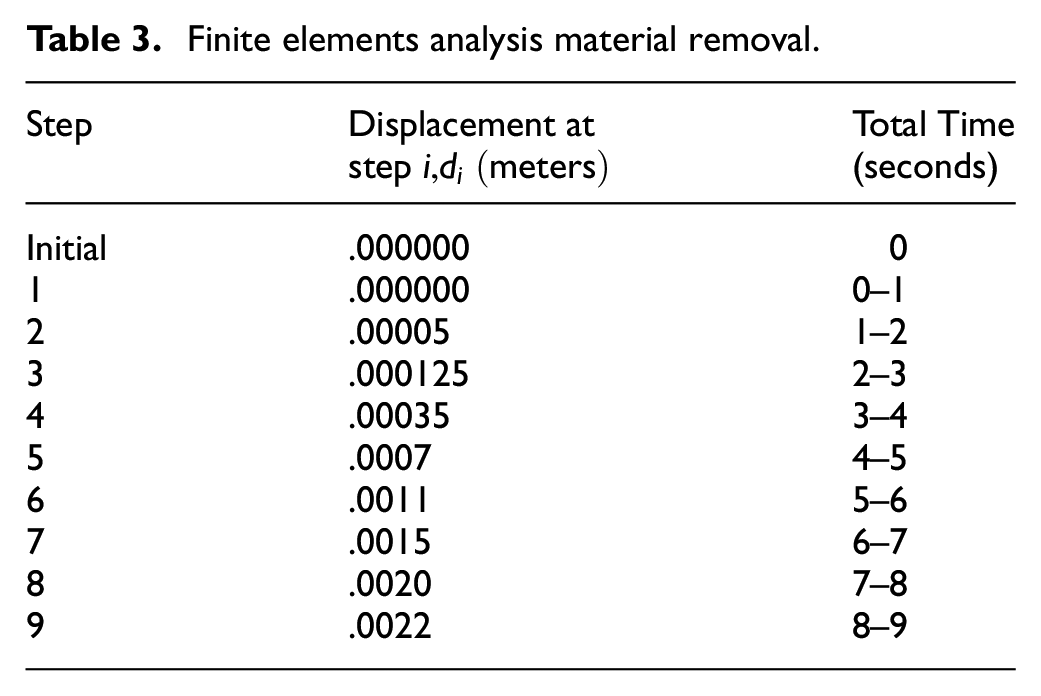
The part in Figure 12 was first partitioned by displacement data at 1 second intervals and thermocouple locations producing the partitions in Figure 13. Partitioning at thermocouple locations ensures that when the part is meshed there will be a node located at the same geometric location as the thermocouples. Therefore, the values at these nodes represent the interpolated approximation of data from the experiment. The values from the data for the displacement partitions in 1 second intervals are given in Table 3. Partitioning at displacement locations accounts for the wear: eight steps were created and after each step the model is changed so that that the elements in the lowest partition are removed from the model to represent the wear. The shape functions were generated using four-node linear heat transfer bilinear quadrilaterals when defining the mesh for the part.
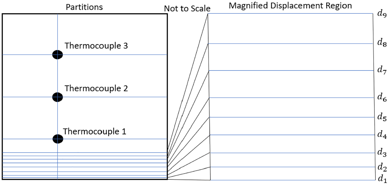
Partitions of the plane model.
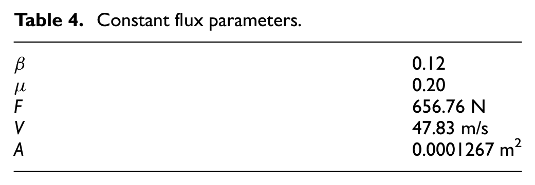
The FEA model was generated using the constant material properties that were defined using Table 1. The heat flux properties are summarized in Table 4 using values from averaging data, or form the assumptions section, as applicable. The plate is given a thickness of
Constant flux parameters.
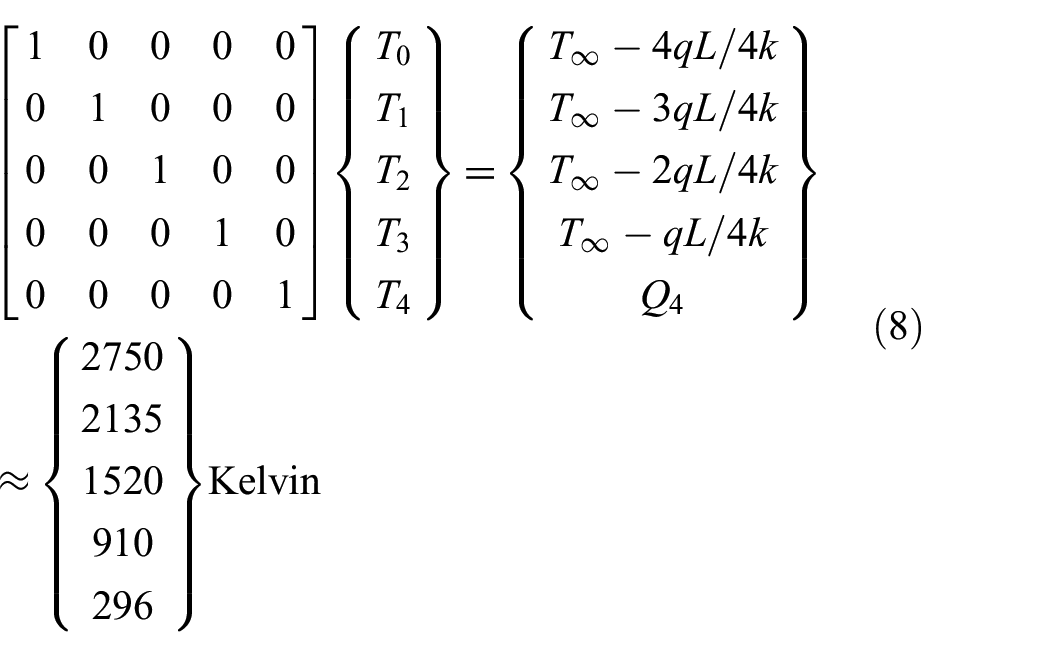
Steady-state solutions were obtained to validate the computer model set up versus the results of Equation (9) and to test for convergence. A coarse mesh containing 96 elements and 117 nodes, a fine mesh containing 728 elements with 783 nodes, and a control mesh of 899 elements with 960 nodes were used to check convergence of the solution. Convergence of the mesh is achieved for the fine mesh of 728 elements. The maximum and minimum values along the bottom boundary were used to determined convergence. The difference in maximum and minimum temperatures between the control and fine mesh are within .0001% of each other, as shown in Figures 14 and 15. The fine mesh is used for all subsequent analysis.
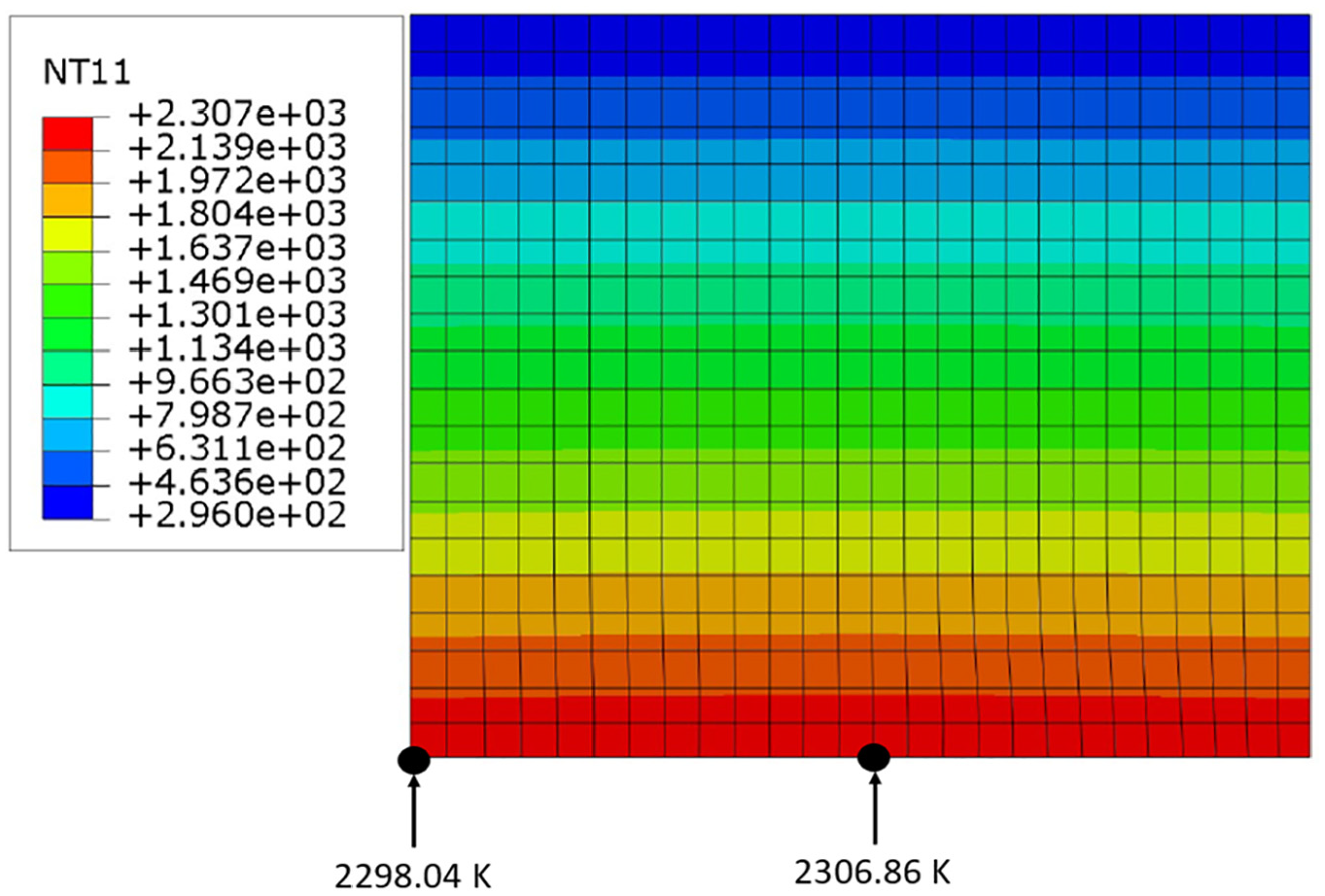
End state of the steady-state FEA model with 793 nodes.
End state of the steady-state FEA model with 960 nodes.
For transient solutions the model seen in Figure 12 is used. Transient steps were implemented in Abaqus 10 using 1 second increments per step, with a moving heat flux boundary corresponding to the displacement data in Table 3. At the end of each 1 second interval the bottom-most remaining partition is removed and the flux is moved to the new bottom-most surface to model the wear. This creates a two-dimensional non-linear, moving boundary, transient FEA model of the pin.
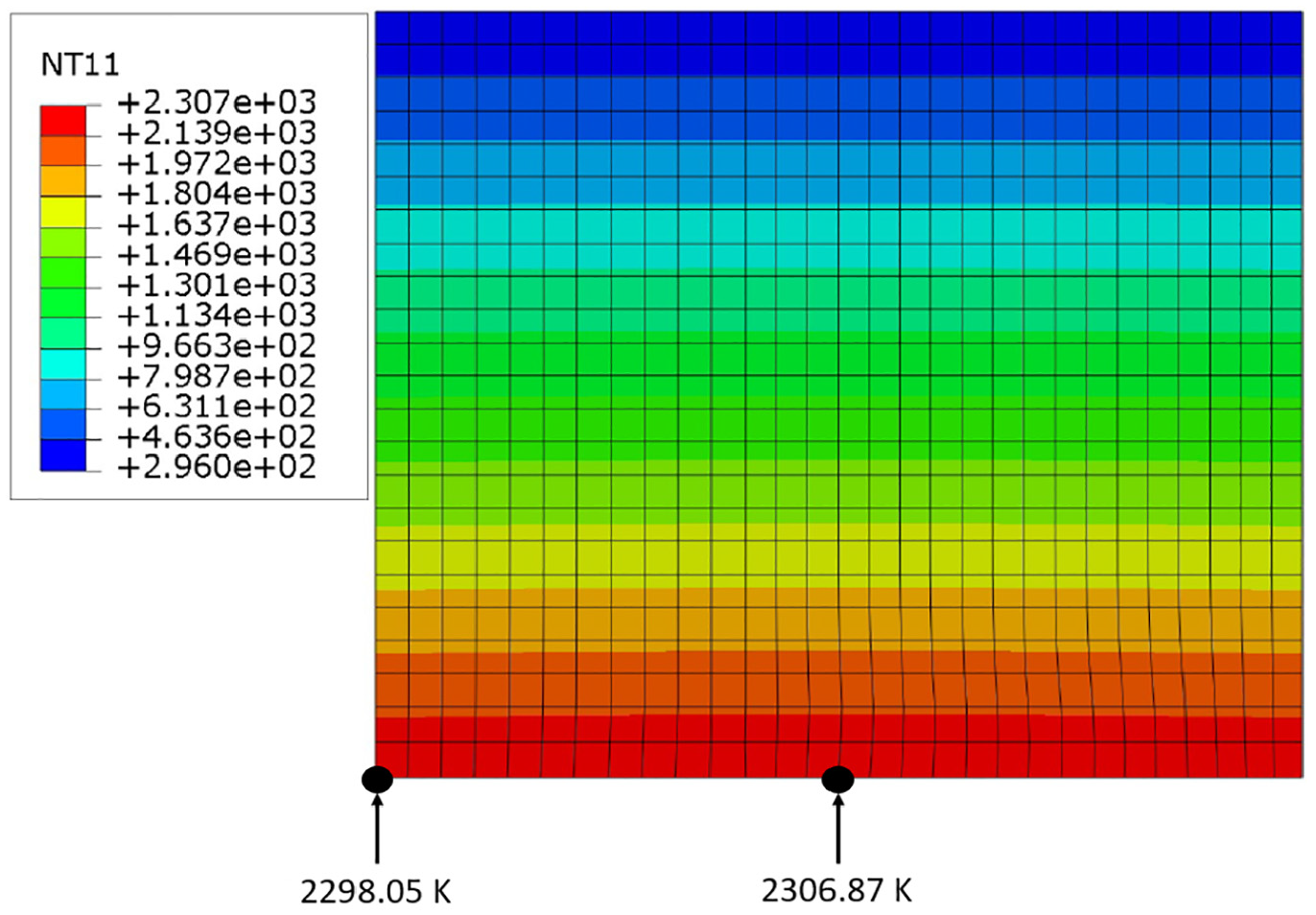
The initialized two-dimensional FEA model is shown in Figure 16. The elements surrounding the three thermocouple locations have been highlighted for reference. Figure 17 shows the removal of the bottom seven partitions and the final state of the model at 8 seconds. The nearly horizontal isotherms were noted, and investigation into the contributions of the convection with the surrounding air was conducted by removing the surface films from the model, effectively creating a one-dimensional representation. The temperature profiles of the two-dimensional and one-dimensional model are shown in Figure 18. The average relative difference between models was found to be less than 1% and so the convection was determined to be negligible in this study.
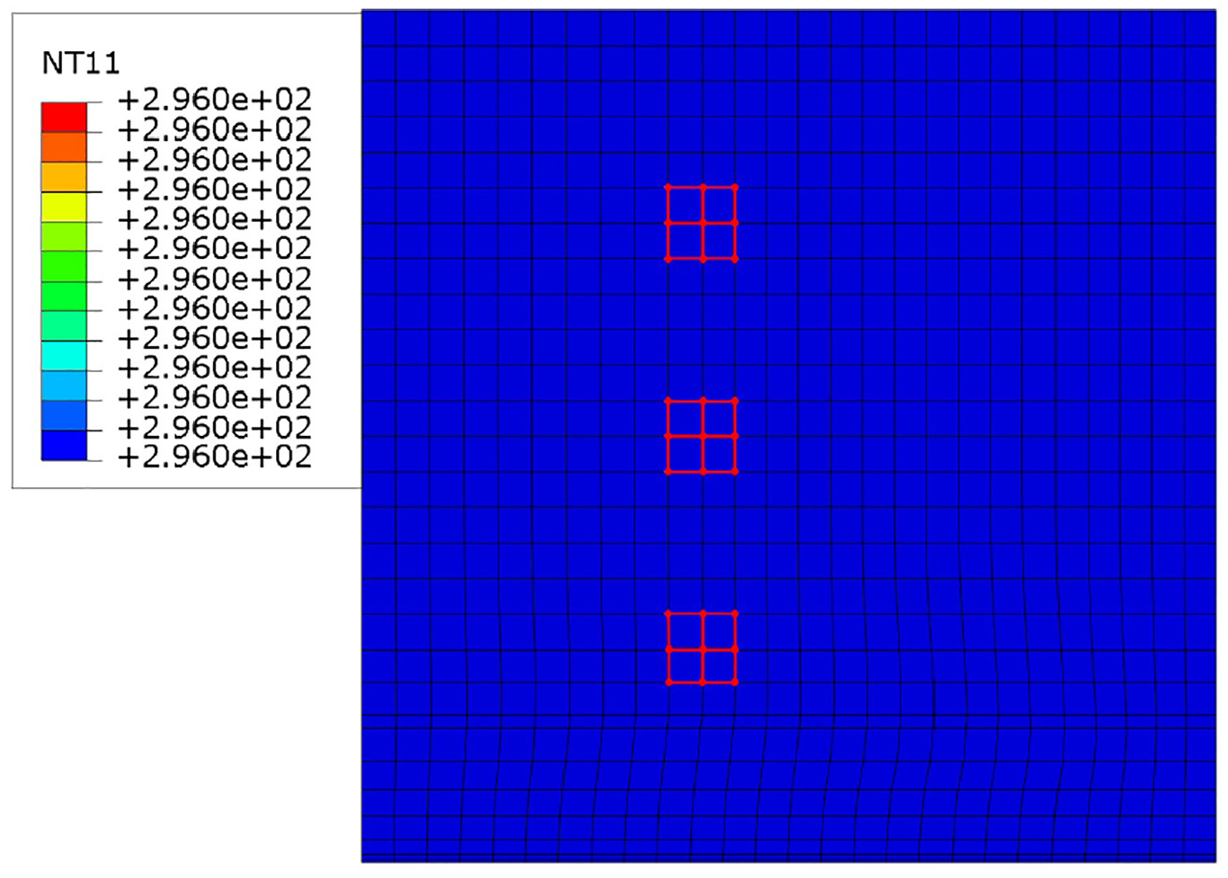
Initial state of the two-dimensional FEA model (t = 0 s).
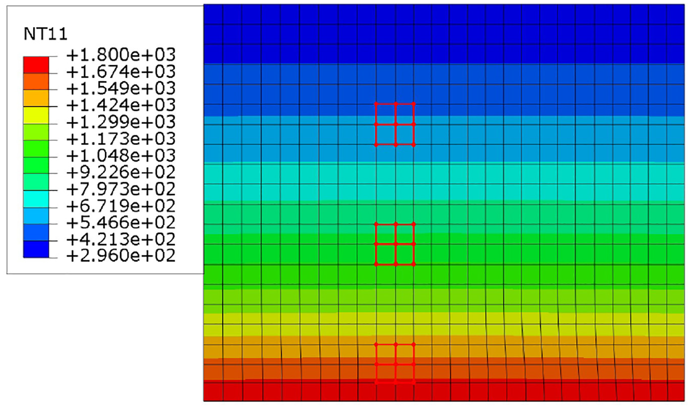
End state of the two-dimensional FEA model (t = 8 s).
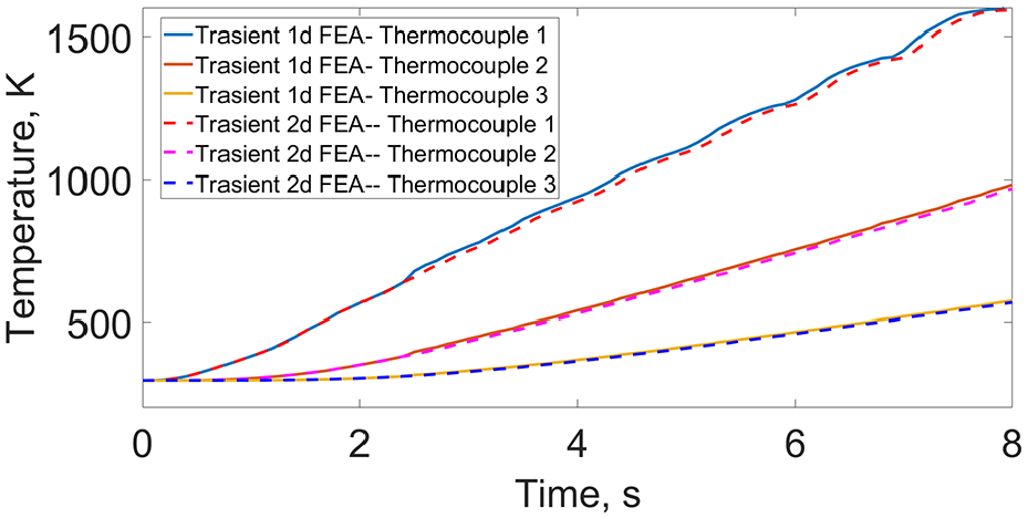
Temperature profiles of thermocouples for 2-D and 1-D FEA models.
The temperature profile of the one-dimensional model is plotted against the data in Figure 19. The model generally trends well with the data, nearly tracing the data for thermocouple 2, but that the model exceeds
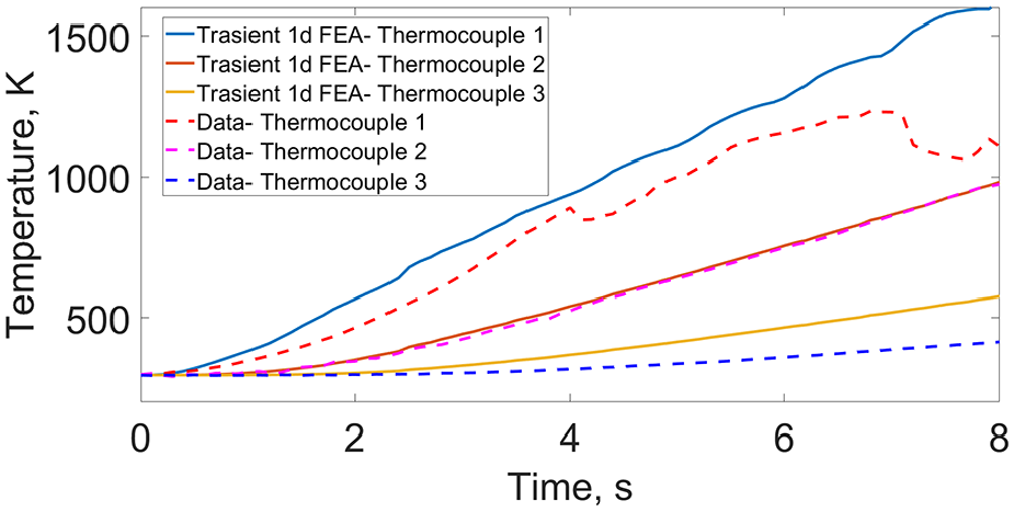
Temperature profiles of thermocouples for 1-D FEA model and the data.
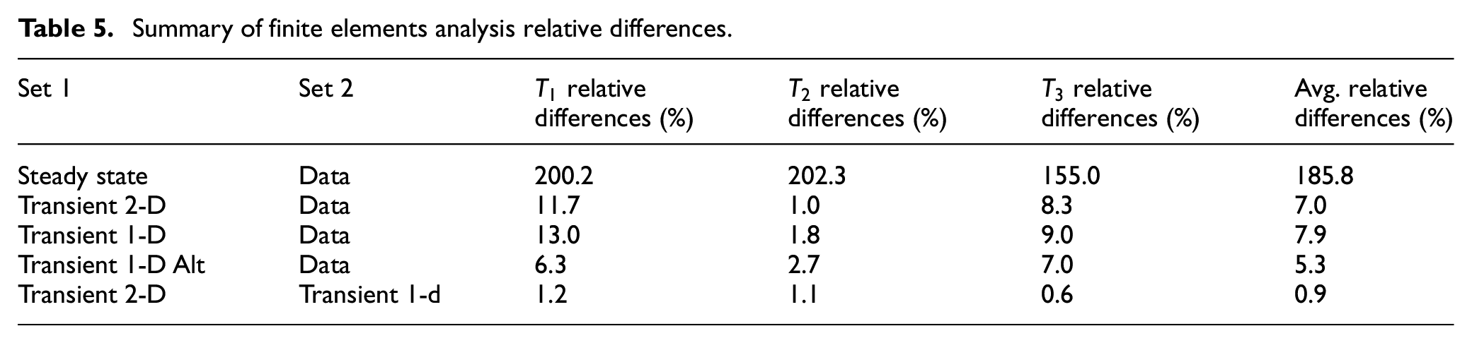
There are many factors involved that could have been changed to lower the temperature at the surface for the model, but this change was taken because it is supported by the way the partition function is trending in Figure 6 and the large Peclet number for this experiment. The temperature profile for this alternate one-dimensional model is given in Figure 20. While thermocouple 2 is no longer traced by the data, the average relative difference between the model and the data is smaller and the temperature at the surface no longer exceeds melt. Table 5 provides a summary of FEA computed average relative difference at thermocouples 1, 2, and 3 labeled here as T1, T2, and T3, respectively.
Summary of finite elements analysis relative differences.
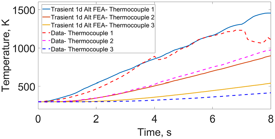
Temperature profiles of thermocouples for the alternate 1-D FEA model and the data.
5. Spectral methods
After determining it appropriate to reduce the model to one-dimension, we decided to implement spectral methods primarily for efficiency. Diffusion of heat through an initially constant temperature cylinder is a problem that results in smooth data on a simple domain. For problems on simple domains, with smooth data, spectral methods provide good approximations. 13
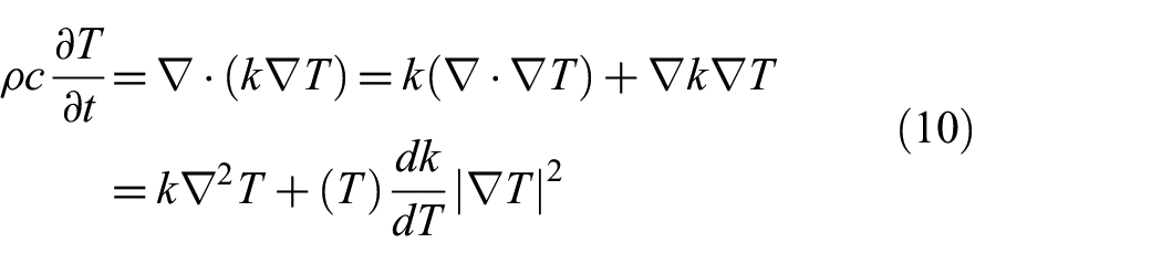
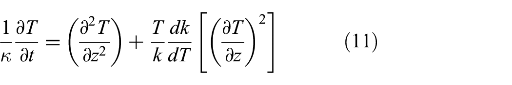
The general form of the heat diffusion equation is given by Equation (10).
14
Transforming to cylindrical coordinates,
3
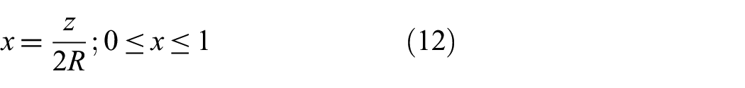
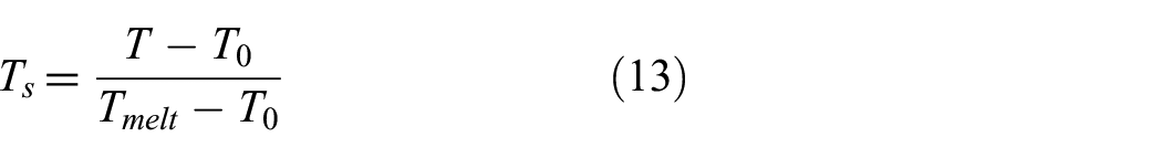
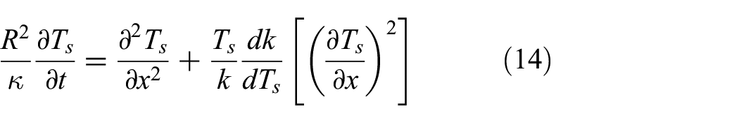
and reducing to one-dimension, results in Equation (11). Redefining the length by Equation (12), and the temperature by Equation (13), results in the scaled heat equation given by Equation (14). The MATLAB cheb command generates a derivative matrix,
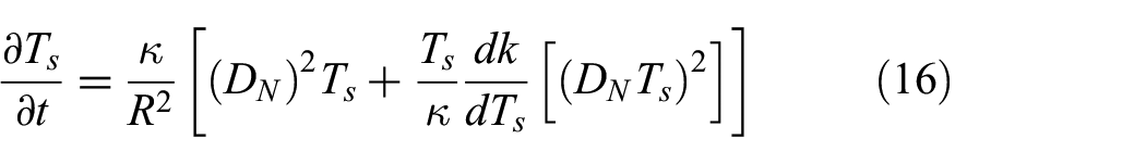

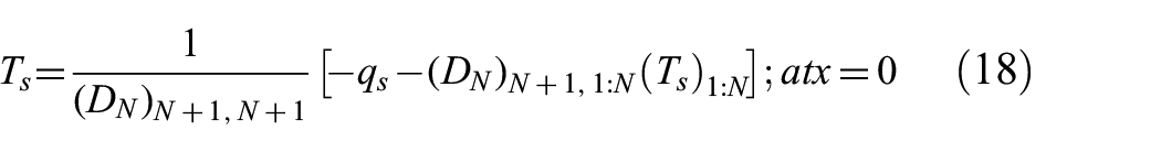
The schematic for the scaled one-dimensional spectral methods model of the pin is shown in Figure 21. The system given in Equations (16)–(18) is completely defined so that the derivative in time can be solved using finite-difference methods. For initial solutions, the MATLAB built-in stiff differential equation solver ode15s
15
was called since the heat equation is known to exhibit stiffness.
16
The moving boundary was defined in the same manner as in the FEA section using the displacement function given by the data in 1 second increments, provided in Table 3. However, the derivative matrix,
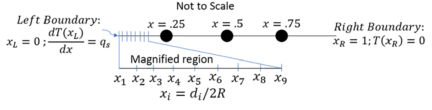
Scaled one-dimensional model of the pin.
In order to satisfy the domain requirements and implement the solution, we rescale each
Spectral method material removal.
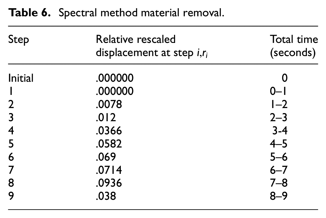
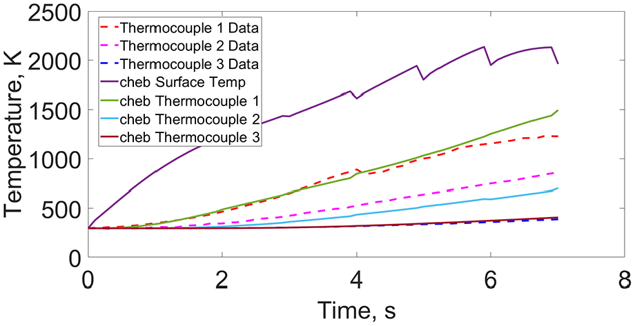
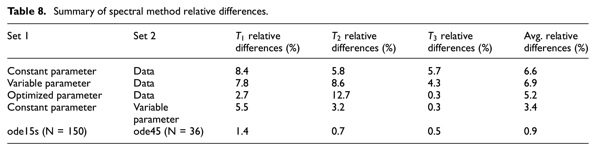
The same constant properties were used as in the one-dimensional FEA case provided in Tables 1 and 3. The rescaled displacements, which model the wear of the pin, and the modeled temperature through the pin are visualized by Figure 22. The resulting temperature profiles of the thermocouples and surface temperature are shown in Figure 23. The average relative difference between the spectral methods model with constant parameters and the data are 6.6%, which is an improvement from the FEA models that also used properties from Tables 1 and 3.
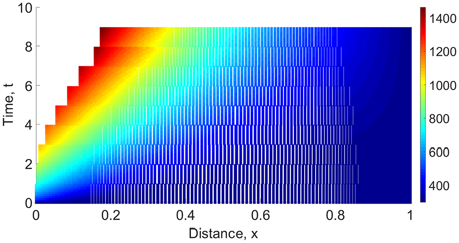
Wear and temperature profiles through the scaled 1-D pin using spectral methods.
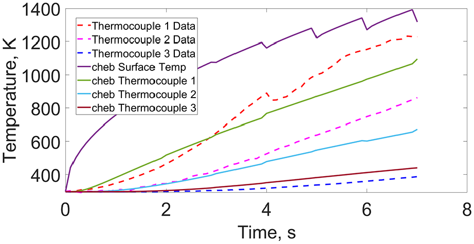
Temperature profiles of thermocouples, surface, and the data using spectral methods.
Variable parameters were also considered by using the fifth order averaged interpolant for the forcing data (shown in Figure 24) and the functional estimate of the thermal conductivity seen as the curve fit of Figure 7.
2
Thermal diffusivity was held constant at
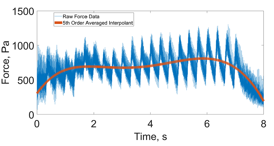
Polynomial interpolant of the raw force data.
Recall that the FEA model was improved by decreasing the partition function, but note that the spectral method does not benefit in the same way. While the FEA model was seen in Figure 19 to be overshooting the data, Figure 23 shows the spectral method model to be generally undershooting the data. To find the model parameters that would make a better fit the data two main factors were considered: how much heat enters the system through friction which was controlled by the value of the product of
A two-dimensional optimization routine was created using the MATLAB function fmincon
18
to determine the optimal values of
Temperature profiles of thermocouples, surface, and the data using optimized spectral methods.
Finally, a convergence study was conducted to investigate the stiffness of Equation (16). Table 7 shows the exponential increase of time-steps and overall time required to solve for the first 1 second of the solution using the MATLAB solver ode45.
19
Equation (16) is determined to be stiff which results in an out of memory error by
Time-steps and time required to solve equation (16) using ode45.
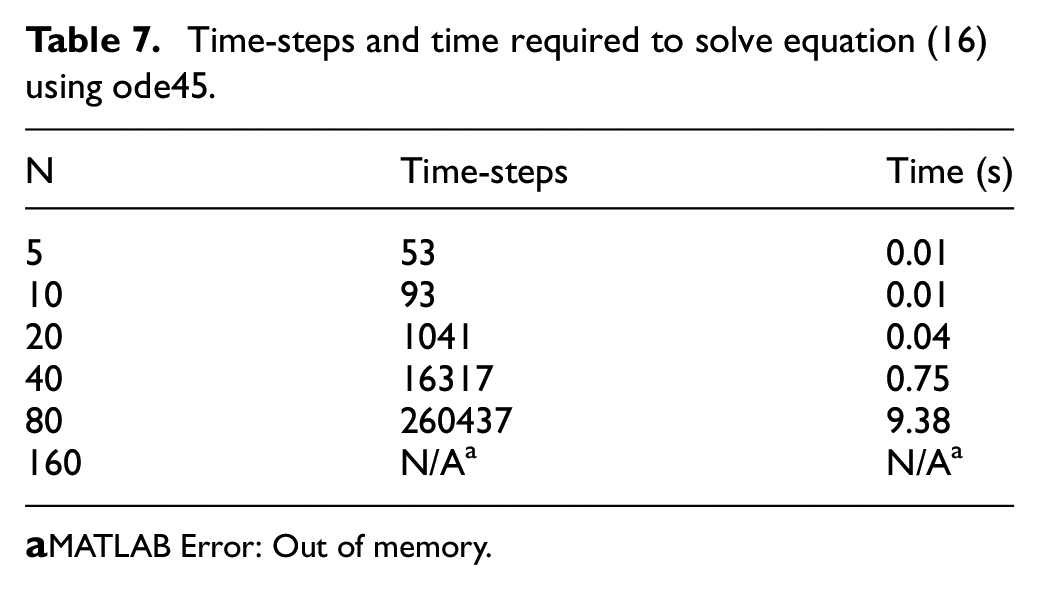
MATLAB Error: Out of memory.
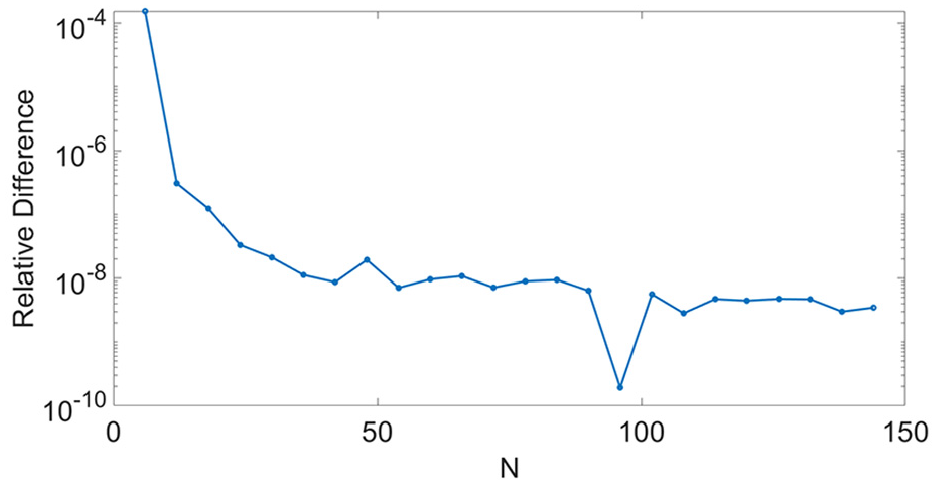
Convergence of ode45.
All previous solutions presented used ode15s with
Summary of spectral method relative differences.
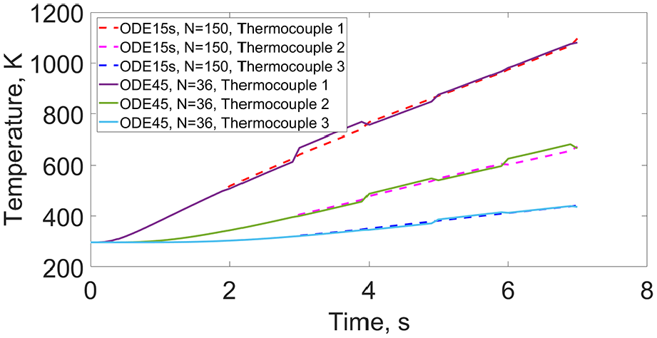
Temperature profiles of thermocouples for the ode15s with N = 150 and ode45 with N = 36 Models.
6. Conclusions
Two separate numerical solutions were generated to solve the non-linear heat equation with a moving boundary, and empirical evidence from a high-speed pin-on-disk experiment was used to provide validation. Finite element analysis and spectral methods each provided unique opportunities to inspect the progression of heat transfer through the pin. The frictional heat source was assumed to be generated uniformly across the pin face and the opposite end of the pin was assumed to maintain the temperature of the ambient air. Finally, assuming uniform convective heat loss off the sides of the pin, the model reduced to two dimensions. Finite element analysis was used to first show that the steady-state solution could not effectively represent the empirical evidence (Equation (8) and Figure 14) so that a transient solution would be required. The transient finite element analysis model then provided insight that the pin experiences negligible heat loss with the surrounding air (Figure 18). Negligible convection effectively reduces the model to one-dimension. The one-dimensional finite element model qualitatively represents the thermocouple data well, as exhibited by the tracing of thermocouple 2 in Figure 19. However, the model over-represents the temperature profile along thermocouples 1 and 3. The finite element analysis was completed using only constant parameters, and analysis into the effect of variable parameters was desired. With the reduction to one-dimension, it was believed that switching to a different solution method would provide a more efficient form to interrogate variable parameters.
Spectral methods, formed via the differentiation matrix, were implemented. As an added benefit, solution times using spectral methods were reduced to about 1 second. The solution profiles of the temperature at the thermocouples using spectral methods qualitatively represent the empirical data well, as exhibited by Figure 23. While thermocouple 2 was virtually traced by the FEA method, the overall representation of the three thermocouples is modeled best by the spectral methods. The introduction of variable parameters does not improve the model qualitatively or quantitatively when using spectral methods, so it is concluded that including variable parameters is not advantageous for this pin-on-disk experiment. Optimizing the parameters provided a
Finite elements analysis and spectral methods both provided good qualitative temperature profiles for the thermocouple temperatures using one-dimension and constant parameters. Spectral methods provided the best quantitative measure of fit by producing an average relative error of 6.6% versus 7.9% using finite elements. Implementing spectral methods for the space derivative also provided the ability to avoid the stiffness presented by the mathematical model; achieving spectral accuracy with a course mesh does not present an issue for the computational efficiency or accuracy of explicit methods for the time derivative.
For future work, extended FEA models and radial basis functions are suggested. The assumptions that were made to reduce the cylindrical pin to a two-dimensional plane model were uniform heat generation across the face of the pin and uniform radial convection with the surrounding air. By extending the finite element model to three dimensions it may be possible to determine if any aerodynamic effects of the spinning wheel significantly affect the model; and, if non-uniform frictional heat generation 5 plays a significant role. The finding that reduced the two-dimensional plane model to one-dimension was that radial convection was negligible in the finite element analysis. Radial basis functions maybe used to generate a derivative matrix with high accuracy and can be easily extended to higher dimensions 20 so that Equation (16) can be solved in two or three dimensions using derivative matrices similarly. Radial basis function-finite-difference (RBF-FD) methods can reduce the derivative matrix to a sparse matrix in the interest of efficiency. 20 Since the size of the matrix will grow exponentially in higher dimensions, it may be of benefit to explore if the computational cost can be reduced by finding an appropriate number of nearest neighbors while adding negligible errors to the solution.
Footnotes
Appendix 1
Funding
The author(s) received no financial support for the research, authorship, and/or publication of this article.