Estimating the tactical impact of robot swarms using a semi-automated forces system and design of experiments methods

Abstract

Militaries are developing autonomous robots to conduct missions such as reconnaissance and surveillance. Some of those robots are intended to operate in swarms. Because operational robot swarms are not yet available, doctrine developers will initially use constructive entity-level combat models to develop and test tactics for robot swarms. Design of experiments methods and retrodiction of the 1991 Battle of 73 Easting between US and Iraqi forces were used to calibrate a semi-automated forces system. The calibrated combat model was then used to estimate the tactical impact of a notional Iraqi robot swarm conducting reconnaissance and surveillance in that battle. The calibration ensured that the model’s parameters were accurate, enabling a reliable estimate of the swarm’s tactical impact. Additionally, the design of experiments methods produced estimates of the interaction of the robot swarm’s effect with the technologies of the combatants’ weapon systems. Simulation trials and statistical analysis showed that the tactical benefits of an Iraqi robot swarm were overshadowed by the advantage provided by the US forces’ thermal sights. However, additional trials indicated that if both sides had been equipped with optical sights only, the early warning provided to the Iraqi forces by a robot swarm could have had a significant effect on the battle’s outcome.

1. Introduction and motivation

As the world enters another period of great power competition, attributes such as autonomy, artificial intelligence, and swarming are increasingly mentioned in the popular media as the future of military technology and doctrine.^1,2,3,4 An application of autonomy, artificial intelligence, and swarming being studied is the use of robot swarms to conduct reconnaissance and surveillance to improve the situational awareness for military forces. The US Army Robotic and Autonomous Systems (RAS) Strategy, published in March 2017, is the Army’s public statement of how the service intends to build on existing robotics capabilities to “achieve unity of effort in the integration of ground and aerial RAS capabilities into Army organizations.” ⁵ Improving situational awareness using Unmanned Ground Systems (UGS) and Unmanned Aircraft Systems (UAS) is one of the five capability objectives of the RAS.

Employing robot swarms in future military operations will require developing swarm tactics that integrate with the capabilities and limitations of a military force’s doctrine, training, and equipment. Tactics are doctrine or procedures for behavior or action at the entity level intended to achieve mission success. Operational examples of military robot swarms are not yet available to develop such tactics in a live environment, nor are there historical examples of military robot swarms. As a result, modeling and simulation will be initially used to develop and test such tactics. ⁶ Doing so necessitates that the model not only accurately represents the capabilities of a robot swarm, but also the human combatants, weapons systems, and the tactics employed by the forces engaged in the battle.

In this study a semi-automated forces (SAF) system was used to estimate the potential tactical impact of a robot swarm. To be clear, the goal of this study was not how to design swarm robots to perform at a certain level, but rather to estimate what effect a robot swarm performing at a certain level might have on a battle. Therefore the simulated robot swarm was assumed to have certain reasonable, even modest, capabilities without regard to how those capabilities might be implemented.

The first task was to calibrate the relevant parameters of the vehicles and weapon systems in the SAF system, such as armor protection, sensor capabilities, and weapons accuracy, to realistic values. Calibration is an iterative process of executing a simulation model, comparing its results to data describing the modeled system, and adjusting the model to increase its accuracy. In this study, the SAF system, or model, was calibrated using retroactive prediction, or “retrodiction,” a method that involves simulating a historical battle and comparing the simulation results to the battle’s historical outcome. The well-documented Battle of 73 Easting, which was fought during the 1991 Gulf War between US and Iraqi ground forces, was used for the calibration. The result of the actual battle was unexpectedly and decidedly one-sided, requiring the calibration to take into account significant differences between the opposing US and Iraqi forces in weapons technology, tactical employment, and troop training.

Formal design of experiments (DOE) methods were used to structure a calibration of the model. Six factors were identified as likely to affect the outcome of the simulated battles, and two levels were set for each factor. A full factorial experimental design with two replicates per level combination required 128 trial simulations of the battle. Of the six factors, the DOE statistical analysis identified three of them, the US use of thermal sights, the armor protection of the M1A1 tank, and a delay in the Iraqi forces occupying their vehicles and preparing to fight, as the most salient impacts on the outcome of the battle.

The delay in occupying the Iraqi vehicles and its effect on the battle’s outcome might have been prevented if a robot swarm was used to provide adequate early warning. An additional 120 experimental trials were conducted to estimate the effect a robot swarm employed by the Iraqi forces might have had on the outcome. Thirty trials were conducted at each of four combinations of two factors: US forces employing or not employing thermal sensors, and the Iraqi forces employing or not employing a drone swarm for early warning. The use of thermal sights allowed the US forces to observe the Iraqis 800 m beyond visual range due to poor weather conditions at the time of the battle, while the Iraqis only had optical sights available. The use of thermal sights negated any advantage of early warning that the swarm may have provided. However, in trials where both forces only had optical sensors available, the use of swarm robots to provide early warning increased US combat vehicle losses by an average of 4.8 vehicles per trial. The results indicated that the effectiveness of the employment of a robot swarm strongly interacts with the different military technologies available.

This paper is structured as follows. Following this introduction, Section 2 provides background information on the primary topics of this study. Section 3 explains how experimental design methods were applied to calibrate a SAF system. Section 4 details the output and analysis of the calibration. Section 5 reports the results of using the calibrated SAF system to simulate and estimate the tactical effect of a robot swarm. Section 6 states the study’s conclusions and describes possible related future work.

2. Background

This section provides brief background explanations of the primary topics of this work: robot swarms and situational awareness; SAF; verification, validation, and calibration of simulation models; DOE; and the Battle of 73 Easting.

2.1. Robot swarms and situational awareness

Swarm robotics has been defined as “the study of how [a] large number of relatively simple physically embodied agents can be designed such that a desired collective behavior emerges from the local interactions among agents and between the agents and the environment.” ⁷ Robot swarms are characterized by autonomy in that the constituent members of a robot swarm are able “to independently compose and select among different courses of action to accomplish goals based on its knowledge and understanding of the world, itself, and the situation.” ⁸ The particular form of artificial intelligence potentially present in robot swarms, swarm intelligence, is defined as coordination and emergent behavior of natural and artificial systems composed of many relatively homogenous individuals that use “simple behavioral rules that exploit only local information” about the environment and other swarm members to produce self-organizing group behavior. ⁹ Natural analogs of robot swarms include swarm intelligence in groups of ants and bees that allows insect colonies to exhibit complex behaviors.

The US Army RAS envisions that increased situational awareness will be a beneficial capability of robotics and autonomy. The definition of situational awareness includes three progressive levels: the perception of status, attributes, and dynamics of relevant elements in the environment; the comprehension or understanding of the meaning of the elements; and the projection of the knowledge of the status and dynamics of the environment to predict future actions. ¹⁰ A UAS swarm conducting reconnaissance and surveillance could give a commander earlier or enhanced awareness of the actions and intentions of the opposing force. The swarm may be able to provide information about the opposing force without putting human scouts at risk and reducing the combat power available to accomplish other tasks. The latter also contributes to the RAS capability to lighten the warfighters’ physical and cognitive workloads. The information collected by the swarm, when coupled with analysis to perceive and project the actions of an opposing force, also supports RAS capabilities to facilitate movement and maneuver and to protect the force. ⁵

2.2. SAF

Combat simulations may include simulated entities (such as tanks, aircraft, or individual combatants) that are generated and controlled by computer software rather than by human crews or operators. The constructive entity-level combat models that generate and control such entities are known as SAF systems. In training applications, SAF systems may be used to generate hostile entities against which human trainees engage in virtual battles or friendly entities that provide a sizeable friendly force to enable a small group of trainees to practice team tactics. In analysis applications, such as testing a revised tactical doctrine or assessing the effect of an enhanced weapon, SAF systems typically are used to generate all of the engaged entities, allowing the analysis scenarios to be executed repeatedly to support statistical analysis without exhausting human operators or crew.

The physical events and phenomena on the battlefield must be modeled within the SAF system. For example, if a SAF vehicle is moving, its acceleration, deceleration, and turn rates on different terrain types must be modeled. Combat interactions also need to be modeled in accordance with the physics of weapon and armor performance characteristics. SAF systems use specialized applied artificial intelligence algorithms to generate the behavior of the entities they control; those entities react autonomously to the changing battlefield situation.^11,12 The generated behavior must be both behaviorally realistic, in that it appears to be similar to human behavior in the same situation, and doctrinally consistent, in that the actions of the SAF-controlled entities are consistent with the tactical doctrine of the military force(s) the SAF is simulating.

Although the SAF software controls the majority of the SAF entities’ actions, SAF systems typically provide an interface that allows a human operator to monitor, and if necessary manually control, the SAF entities’ behavior. Figure 1 shows an example of a typical SAF operator interface. The SAF system seen in the figure is VR-Forces, a SAF system that is a commercial product of VT MAK. ¹³ VR-Forces has been used for a wide range of training and analysis applications and has an active user community.

Figure 1.

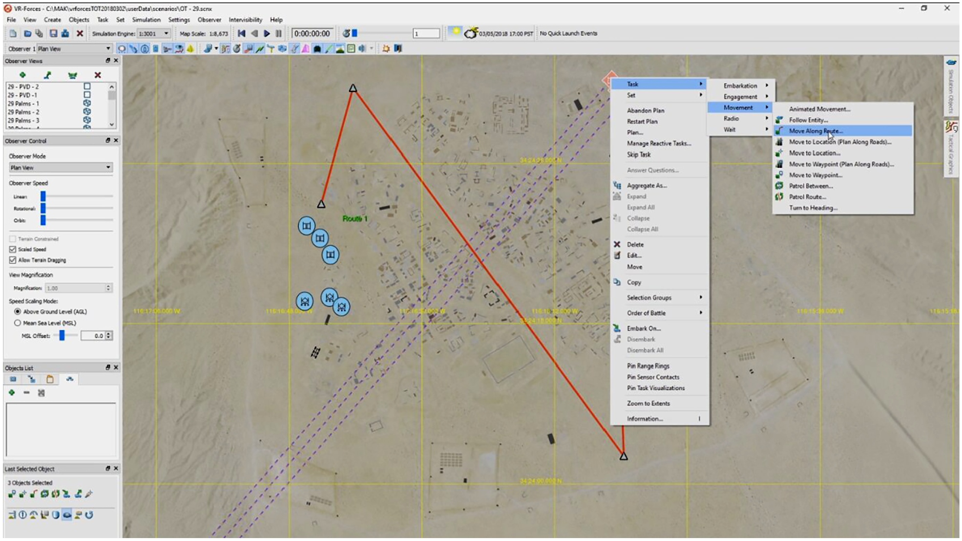
Example SAF system operator interface for VR-Forces. (Image courtesy of MAK Technologies.)

2.3. Verification, validation, and calibration

Verification and validation are essential prerequisites to the credible and reliable use of a model. A model that has not undergone verification and validation is at best useful as a classroom example, and at worst, has the potential to be dangerous if decisions are made based on incorrect model outputs. Verification is the process of determining that a model’s implementation accurately represents the developer’s conceptual description and specifications. ¹⁴ Validation is the process of determining the degree to which a model’s behavior or outputs accurately represent the system or phenomenon it models, from the perspective of the intended uses of the model. ¹⁴ A wide range of model verification and validation methods are available; the appropriate method(s) to use for a particular model depends on the modeling method and the data available.^15,16,17 Finally, calibration is iteratively comparing the model and its results to data describing the system or phenomenon being modeled and revising the model to improve its accuracy. ¹⁸ Calibration is closely related to validation, as the comparisons of model results to reality in calibration are often made using validation methods.

Because they are models, SAF systems must undergo verification and validation. Methods to do so include both adaptations of existing methods and SAF-specific methods.^19,20,21 The calibration of SAF systems also has SAF-specific considerations. ²² One method useful for both validation and calibration of SAF systems is retroactive prediction or retrodiction. In retrodiction, a well-understood historical event, typically a battle or engagement, is modeled using a SAF system to assess the SAF system’s accuracy in terms of how closely it replicates the event’s historical outcome. ²³ Retrodiction can be problematic when the historical event’s outcome was unexpected or unlikely.

2.4. DOE

DOE is a statistics-based methodology for organizing experimental trials. DOE attempts to achieve several potentially competing goals simultaneously: (1) extract as much information from as few experimental trials as possible; (2) satisfy the assumptions of the statistical methods that will be used to analyze the results of the experiment; (3) estimate the portion of variability in the results due to each source of variability; and (4) distinguish the variability in the results due to the conditions of interest, even when other sources of variability are present.

DOE is a broad topic, and even a cursory tutorial is well beyond the scope of this paper; excellent introductions are available.^24,25 Only a few key DOE terms needed for this paper will be defined. A factor is an input independent variable that the experimenter will control during the experiment in order to determine its effect on an output dependent variable in the results; the latter may also be referred to as a response variable. A level is a specific value for a factor that will be used in an experiment. A full factorial design includes at least one trial for every possible combination of factor levels. A DOE model (not to be confused with a simulation model) is a statistical model that describes the data from an experiment. ²⁵ Factors interact when one factor’s level influences another factor’s effect on a response variable. Finally, a replicate is a trial repeated with the same factor levels.

2.5. Battle of 73 Easting

The Battle of 73 Easting, which was influential in the overall outcome of the 1991 Gulf War, was fought on 26 February 1991 in featureless desert terrain near the Iraq–Kuwait border.^26,27 With no nearby town or river to lend its name, the battle was named after a north-south map reference grid line, 73 km east of an arbitrary origin point, near which much of the action took place.

The battle was fought between the 2nd Armored Cavalry Regiment (2ACR) of the United States Army and two brigades of the Tawakalna Division of the Iraqi Republican Guard. Three troops (companies) of 2ACR were most heavily engaged: Iron, Eagle, and Ghost, each consisting of approximately 130 troopers equipped with 13 M3 Bradley fighting vehicles and nine M1A1 Abrams main battle tanks.^28,29

The two Iraqi brigades, the 18th Mechanized Brigade and the 9th Armored Brigade, each consisted of approximately 2500 to 3000 soldiers equipped with approximately 166 T-72 main battle tanks and 158 armored personnel carriers (APC); the latter included both BMP-1 infantry fighting vehicles (IVFs) and other APCs. ³⁰ The Iraqi forces were deployed in several prepared defensive positions along a roughly 10 km stretch of the desert. The battle began around 4:10 pm local time when 2ACR’s Eagle troop, led by then-Captain H. R. McMaster, began moving eastward from near the 67 Easting. Eagle, Ghost, and Iron troops, supported by Killer troop, fought their way through several successive Iraqi positions and later repelled multiple Iraqi counterattacks. During the six-hour battle, 2ACR completely defeated the two Iraqi brigades, destroying at least 133 Iraqi tanks. ²⁸

The simulation study conducted for this research is based on the portion of the battle that occurred in the Eagle troop sector. Figures 2 and 3 show a portion of a VR-Forces simulation of the battle. Eagle troop employed nine M1A1 tanks, 13 M3 Bradley fighting vehicles, and several ancillary vehicles to destroy 50 T-72 tanks, 25 APCs, and numerous other vehicles in a brisk engagement that lasted approximately 23 minutes.^28,29,31 The simulation scenario includes a total of 27 vehicles from Eagle troop (depicted as circular icons in Figures 2 and 3) and 122 Iraqi entities (depicted as diamond and pentagonal icons).

Figure 2.

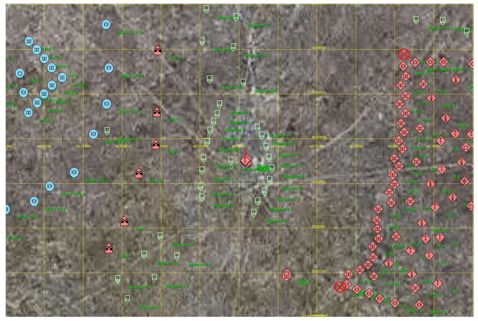
Screenshot of the initial deployments in a VR-Forces simulation of the Battle of 73 Easting. The circle icons represent US vehicles and the diamond and pentagonal icons represent Iraqi vehicles. The seven westernmost Iraqi icons are the notional UASs that constitute the robot swarm; they were not present in the historical battle. (Image courtesy of MAK Technologies.)

Figure 3.

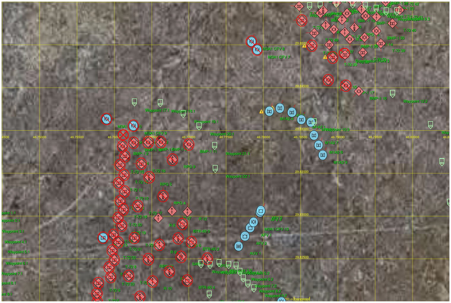
Screenshot of a VR-Forces simulation of the Battle of 73 Easting, approximately midway through the battle. The US forces have already passed through the first Iraqi battle position from west to east and are engaging the second. A circle with a slash over a vehicle icon indicates that the vehicle is destroyed. (Image courtesy of MAK Technologies.)

The locations of the Eagle troop attack axes and the Iraqi fighting positions were determined from Military Grid Reference System coordinates and then converted to align with the VR-Forces terrain model. ³²

3. Calibration experiment design

This section explains how experimental design ideas were applied to calibrate VR-Forces. The calibration objective, the experiment factors, the response variable, and the experiment design and execution are all described.

3.1. Calibration objective

Calibration, as defined earlier, is adjusting a model to increase its accuracy. For this study VR-Forces was calibrated using the Battle of 73 Easting. Once the model was calibrated, it could then be used to reliably estimate the effect of a robot swarm on the battle’s outcome.

The Battle of 73 Easting is unusually well documented,^28,33 has been intensively studied for lessons learned, ³¹ and has been the subject of multiple simulation projects.^22,32,34 However, attempts to validate SAF systems using the Battle of 73 Easting as a reference scenario for retrodiction have not been entirely successful. ²² SAF systems often produce much higher losses for the US forces in the simulated battles than actually occurred in the historical battle. ²¹ This suggests that essential aspects of the actual battle that contributed to its one-sided outcome are not adequately represented in SAF systems. SAF systems can fairly accurately model relative differences in the capabilities of sensors and weapons. However, modeling battlefield aspects that may contribute to an unexpected or one-sided outcome, such as intangible attributes (e.g., leadership and professionalism), or interactions among multiple performance parameters (e.g., a design trade between a lower vehicle profile and a slower reload time), are more complicated. Earlier work addressed these difficulties by applying DOE methods to calibrate the VR-Forces SAF system so that it could accurately replicate the actual outcome of the Battle of 73 Easting. ³⁵ This study improves on that earlier work^22,35 by explicitly incorporating technological considerations that might have contributed to the one-sided outcome of the battle, specifically the US use of thermal sights on the M1A1 tank and the M3 Bradley Cavalry Fighting Vehicle, and the superior armor protection on the M1A1 tank as additional factors.

3.2. Experiment factors

This section explains the historical conditions used to identify the experimental factors that represent plausible reasons for the differences between the US and Iraqi performances in the battle.

Six factors were identified for the experiment design as likely to affect the outcome of the simulated battles. Four factors (B, D, E, and F) were selected based on previous simulations of 73 Easting using VR-Forces. ³⁵ Two additional factors, US use of thermal sights and the superior armor of the M1A1 tank, were also included to more closely model the historical accounts of the battle. For consistency, low levels of each factor are defined to favor US forces, while a high factor level favors Iraqi forces. The six factors were:

• A: US thermal targeting systems

• B: T-72 armor protection (P_k)

• C: M1A1 armor protection (P_k)

• D: T-72 probability of hit (P_h)

• E: BMP-1 probability of hit (P_h)

• F: Iraqi time delay vs. robot swarm early warning

Factor A: US thermal targeting systems

Both the US M1A1 tank and the M3 Bradley Cavalry Fighting Vehicle were equipped with thermal targeting systems as well as standard visual optical sights. Thermal sights detect infrared emissions to develop images of targets from the heat generated by the target. The weather conditions during the Battle of 73 Easting were poor as the US forces were emerging from a sandstorm to the west of the battle area that caused hazy conditions. Early simulation studies of the battle based on an inspection of the battlefield and interviews with the US participants from the 2ACR in the weeks immediately after the conclusion of the Gulf War indicated that due to the poor weather conditions during the battle, combat vehicles could be identified at a maximum range of approximately 800 m using the standard visual optical sights that both US and Iraqi vehicles possessed. The additional thermal sights on the M1A1 and M3 provided the US forces with the ability to identify Iraqi vehicles at a range of approximately 1600 m, conferring a significant tactical advantage to the US forces.^32,36 The simulation entities representing M1A1 tanks and M3 Cavalry Fighting Vehicles are equipped with both thermal and optical sights at the low level of this factor. At the high level of the factor, simulation entities representing M1A1 tanks and M3 Cavalry Fighting Vehicles have only visual sights, giving them equal visibility with their Iraqi opponents. Thermal and optical sights were configured with effective ranges of 1600 and 800 m, respectively.

Factor B: T-72 armor protection and factor C: M1A1 armor protection

The probability of kill (P_k) is the probability of a fired round destroying its intended target, assuming that it hit the target. P_k values may depend on the weapon, the type of round, the range, and the target’s armor. The armor protection of the T-72 is both less thick and of lower material quality than that of the M1A1. Some T-72s were destroyed by a single hit from M1A1 120 mm armor-piercing discarding sabot (APDS) ammunition, and others by one or two hits from high explosive anti-tank (HEAT) ammunition designed to engage light armor vehicles such as the BMP-1. ²⁸ Further, T-72s were also destroyed by the 25 mm gun from the M3 Bradley when an M3 engaged the T-72 from the side or rear of the tank, where armor protection is not as robust. Some M3s fired a hundred rounds or more from their 25 mm gun to set a T-72 on fire. ²⁸ On the other hand, the high quality of the M1A1 Chobham composite armor, as well as the low quality of the T-72 125 mm APDS ammunition, resulted in the M1A1 being able to survive direct hits from T-72s.

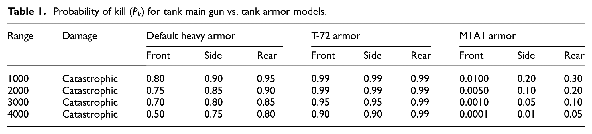
VR-Forces provides two default armor settings, “light armor” and “heavy armor.” In addition, the model provides two methods to customize the effect of armor protection. One method is a physics-based model of the ammunition and the armor, while the other allows the direct assignment of probability of kill given a hit (usually abbreviated as P_k) for vehicle entity models when engaged by specific ammunition types at different ranges between the firing vehicle and the target. ¹³ This study included three custom models of heavy armor protection using direct assignment of P_k for vehicle entity models. The first model is a “default heavy armor” model that uses P_k values used in the “heavy armor” setting in the VR-Forces versions used in earlier work.^22,35 The second armor protection model reflects the vulnerability of T-72 armor displayed in the historical record. The third armor protection model corresponds to the exceptional performance of the M1A1 armor during the 1991 Gulf War. Table 1 shows the P_k values at different ranges for the different armor models when engaged by an APDS round. Table 2 shows the P_k values at different ranges for the different armor models when engaged by the smaller guns on the IVFs (the M3 Bradley and the BMP-1). For factor B, T-72 armor protection (P_k), the low level is the T-72 armor damage model, and the high level is the default heavy armor model. For factor C, M1A1 armor protection (P_k), the high level is the default heavy armor model, while the low level is the M1A1 armor damage model. For both factors, the low level favors US forces and the high factor level favors the Iraqi forces. Both factors include a set of P_k values of HEAT ammunition, but the values are not reported here because the first choice of ammunition type for a tank to engage an opposing tank is APDS. A firing tank in the simulation will ordinarily use HEAT rounds to engage IFVs, only using HEAT rounds against tanks when it has no remaining APDS rounds.

Table 1.

Probability of kill (P_k) for tank main gun vs. tank armor models.

Range	Damage	Default heavy armor			T-72 armor			M1A1 armor
		Front	Side	Rear	Front	Side	Rear	Front	Side	Rear
1000	Catastrophic	0.80	0.90	0.95	0.99	0.99	0.99	0.0100	0.20	0.30
2000	Catastrophic	0.75	0.85	0.90	0.99	0.99	0.99	0.0050	0.10	0.20
3000	Catastrophic	0.70	0.80	0.85	0.95	0.95	0.99	0.0010	0.05	0.10
4000	Catastrophic	0.50	0.75	0.80	0.90	0.90	0.99	0.0001	0.01	0.05

Table 2.

Probability of kill (P_k) for M3 Bradley and BMP-1 guns vs. tank armor models.

Range	Damage	Default heavy armor			T-72 armor			M1A1 armor
		Front	Side	Rear	Front	Side	Rear	Front	Side	Rear
1000	Catastrophic	0.0002	0.002	0.010	0.001	0.01	0.05	0.0001	0.001	0.005
	Firepower	0.0050	0.01	0.020	0.025	0.05	0.10	0.0025	0.005	0.01
	Mobility	0.0050	0.01	0.020	0.025	0.05	0.10	0.0025	0.005	0.01
2000	Catastrophic	0.00015	0.0015	0.0075	0.00075	0.0075	0.0375	0.000075	0.00075	0.00375
	Firepower	0.00375	0.0075	0.015	0.01875	0.0375	0.075	0.001875	0.00375	0.0075
	Mobility	0.00375	0.0075	0.015	0.01875	0.0375	0.075	0.001875	0.00375	0.0075
3000	Catastrophic	0.0001	0.001	0.005	0.0005	0.005	0.025	0.0005	0.0005	0.0025
	Firepower	0.0025	0.005	0.010	0.0125	0.025	0.05	0.00125	0.0025	0.005
	Mobility	0.0025	0.005	0.010	0.0125	0.025	0.05	0.00125	0.0025	0.005

Factor D: T-72 probability of hit and factor E: BMP-1 probability of hit

The probability of hit (P_h) is the probability of a fired round hitting its intended target. In VR-Forces, P_h can be set by the user for each weapon system and can be range-dependent, i.e., P_h is usually lower at longer ranges. The default VR-Forces values for T-72 and BMP-1 P_h were the same as for the US M1A1 Abrams and M3 Bradley. ¹³ In an earlier attempt to retrodict 73 Easting, the P_h values for Iraqi T-72 tanks and BMP-1 fighting vehicles were substantially reduced to P_h values of less than 10% at even the closest ranges, ²² a reduction that could be considered questionable. Initial experiments in this study that included US thermal sights and the armor protection models described earlier for factors A, B, and C indicated that the P_h values could be set at more realistic values and still produce results consistent with the historical record. The reduced value for the T-72 P_h modeled the difference in soldier skill and equipment performance between the US and Iraqi armies. ²² The reduced value for the BMP-1 P_h modeled the shorter range of its low-velocity 73 mm gun as compared with the M3 Bradley’s high-velocity 25 mm gun. Additionally, the BMP-1 gun is manually loaded and the vehicle carries only 40 rounds of ammunition, whereas the M3 Bradley gun is a rapid-firing chain gun supplied with 1500 rounds of ammunition on the vehicle. The levels for factors D and E are displayed in Table 3. While not a factor that varies in the model, the P_h values for the M1A1 120 mm were adjusted to a higher level than the default level for tanks to reflect the superior capabilities of the gun’s targeting system, which includes a laser range finder and a computer to adjust the firing solution given the range of the target. With the thermal sight and the targeting system, during the Gulf War M1A1s achieved first-round kills at ranges of up to 4000 m. ³⁷

Table 3.

Probability of hit (P_h) for the T-72 125 mm gun (factor D), the BMP-1 73 mm gun (factor E), and the M1A1 120 mm gun.

T-72 125 mm gun			BMP-1 73 mm gun			M1A1 120 mm gun
Range	Ph High	Ph Low	Range	Ph High	Ph Low	Range	Ph
1000	0.90	0.45	500	0.80	0.40	1000	0.99
2000	0.80	0.40	1000	0.60	0.30	2000	0.95
3000	0.70	0.35	1500	0.30	0.15	3000	0.90
4000	0.50	0.25	2000	0.10	0.05	4000	0.80

Factor F: Iraqi time delay vs. robot swarm early warning

When the actual battle began, most of the Iraqi tank crews were taking shelter in bunkers to avoid potential US air attacks, and they had to run from the bunkers to their tanks after the US forces had already begun firing. ³⁴ Moreover, some Iraqi soldiers not in the bunkers may have believed the initial explosions from the incoming tank rounds were instead from air attacks, briefly causing them to run to the bunkers instead of their vehicles.^32,34 Consequently, the US forces would have had a distinct advantage for the first 1–2 minutes of the engagement before many Iraqi crews were ready to fight. The low level of factor F was a delay of two minutes between the time US entities destroyed the first Iraqi vehicle in a battle position and when the Iraqi entities in that battle position could return fire. The delay was implemented in VR-Forces using a scenario script controlling the Iraqi forces. The high level of factor F was no time delay, i.e., the Iraqi vehicles could fire as soon as they sighted a target. It was implemented by including in the scenario seven entities composing a swarm of robot UASs. The robot swarm was intended to provide sufficient warning of the approach of US ground forces to allow the Iraqi crews to occupy their vehicles before the US vehicles were within visual range. If any of the robots spotted a US entity, a simulated radio message was transmitted to the Iraqi entities and the scenario script controlling the Iraqi forces would turn off the delay.

3.3. Response variable

Because the goal of the calibration was to correct the unrealistically high US losses in SAF simulations of 73 Easting, as compared with the historical outcome, the number of destroyed U.S. vehicles was selected as the response variable. Considering only a single response variable risks neglecting important qualitative differences in the simulation outcomes, e.g., which side won the battle, but this calibration was focused on reducing the number of destroyed US vehicles to the historical level.

For the sake of generality and consistency with much of the simulation literature, hereinafter we switch from specific references to the “US” and “Iraqi” to generic references to “Blue” and “Red,” respectively. Thus the response variable, for example, will be referred to as “Blue destroyed” rather than “US destroyed.”

3.4. Experiment design and execution

One goal of DOE is parsimony in number of trials required, i.e., to extract as much information as possible from as few trials as possible. A power analysis was used to determine the minimum number of replicates required to obtain the desired statistical power.

For the main experiment, a full factorial 2⁶ experimental design with two replicates was used. In other words, there were six factors with two levels each, giving 2⁶ = 64 possible combinations of factor levels. Minitab’s power analysis function was used to estimate the number of replicates (trials or simulations) that would be needed to detect a difference of five in the mean Blue destroyed for the six-factor, two-level experiment. A difference of five was chosen based on pre-experiment simulations of 73 Easting with VR-Forces; 32 such simulations had averaged 52% Blue destroyed, compared with the calibration target of less than 5%. ³⁵ Therefore, substantial differences between opposing response-factor combinations were needed, and detecting subtle differences was not necessary. The same pre-experiment simulations produced a standard deviation s = 8.5270 for Blue destroyed, which was used as the estimated standard deviation for the power analysis. At α = 0.05 and a minimum power of 0.9, Minitab’s power analysis calculated that 128 total trials with two replicates of each of the 64 factor combinations to detect an effect of 5.0 would produce an actual power of 0.9963, exceeding the objective of the power analysis.

The trials were executed using the VR-Forces software. Because all of the trials were run on the same computer by a single experimenter, there were no potential “nuisance factors” that required a blocking design.

4. Calibration results and analysis

This section reports the results obtained by running the calibration experiment as designed using the VR-Forces software.

4.1. The 2⁶ model

The results obtained from the 2⁶ design were used to determine which factors and interactions had the strongest effect on the response variable, Blue destroyed. The factors and interactions with statistically significant effects would then be retained to build a reduced model.

The results (Blue destroyed) obtained from the 128 trials of the 2⁶ design were analyzed using an analysis of variance (ANOVA) with full interactions down to all six interaction levels in order to obtain a normal probability plot of standardized effects. The intent was to identify the input variable(s) that were most likely to be statistically significant. The level of significance was set to α = 0.10 to capture all factor combinations that might be significant at α = 0.05 in the reduced model.

Figure 4 is a scatterplot of Red losses versus Blue destroyed over the 128 trials that were executed; each trial is one simulation of the battle. In the figure, circles are trials where Blue forces did not have thermal sights (factor A high), and the Red forces had early warning due to employing a robot swarm, thereby avoiding a delay (factor F high). The plot indicates a strong interaction between factors A and F. All of the trials where Blue destroyed exceeded 50%, including those trials where Red essentially won the battle by inflicting a higher percentage loss on Blue than suffered by Red, are cases where both factors A and F favored the Red forces. Table 4 is a summary of the descriptive statistics for Blue destroyed. The losses range from zero Blue destroyed (the historical result) and 27 Blue destroyed (100%). The box plot in Figure 5 shows that most of the trials had Blue destroyed that were close to the median value of 5, but that 14 trials were outliers with high Blue destroyed. All of the outlier values for Blue destroyed were combinations of factors A and F both high.

Figure 4.

Scatter plot of the results of the 128 trials used in calibration with Blue destroyed on the x-axis and Red losses on the y-axis. The legend indicates combinations of factor A (Blue thermal sights) and factor F (Red delay).

Table 4.

Descriptive statistics for the calibration trials.

Variable	n	Mean	SEmean	Stddev	Variance	Min	Q1	Median	Q3	Max
Blue destroyed	128	7.039	0.654	7.400	54.762	0.000	1.250	5.000	9.000	27.000

Figure 5.

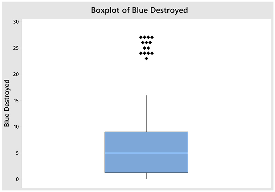
Box plot of the Blue destroyed for the 128 trials used in calibration. Diamonds indicate outliers.

Figure 6 is a normal probability plot of the standardized effects for the full 2⁶ DOE model with all interactions. The response variable is Blue destroyed, and the significance level is α = 0.10. In the figure, circles indicate that the effect is not significant, whereas squares indicate that the effect is significant. The figure shows that factors A, B, C, D, and F were statistically significant. Factor E (BMP-1 P_h) was not statistically significant. The AF, CF, ACF, AC, AD, BDE, CD, ACD, BDE, and ABCE interactions are statistically significant at α = 0.10 and should remain in the DOE model. Note that the most substantial effects for the interactions AF, CF, and ACF all are combinations that include the Red delay. The Red delay (factor F) is significant and interacts strongly with Blue thermal sights (factor A) and M1A1 armor protection (factor C).

Figure 6.

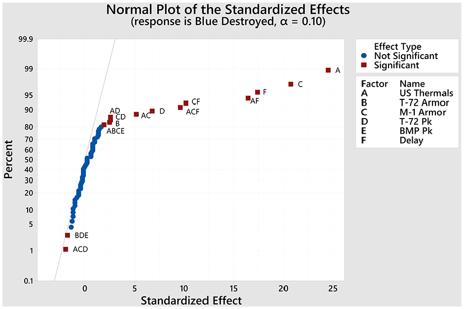
Normal probability plot of the standardized effects for the 2⁶ model with all interactions. The level of significance is α = 0.10 for the response variable Blue destroyed.

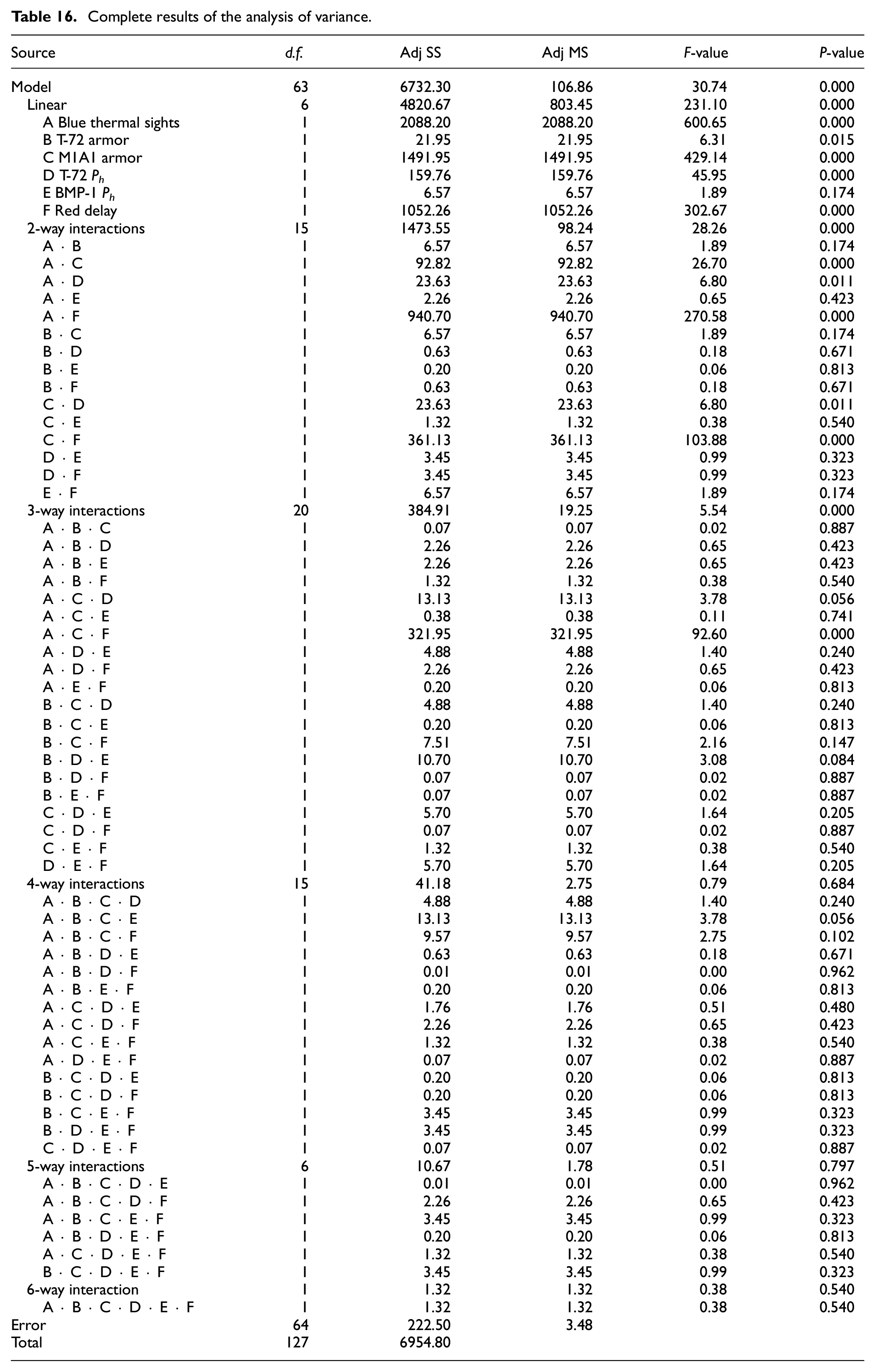
The ANOVA output, which is reported in detail in Table 16 of the Appendix, shows that the model is statistically significant with an F-value of 30.74 and a P-value of < 0.0005. Based the results of the ANOVA, as shown visually in Figure 6, the reduced model included factors A, B, C, D, and F as well as the AC, AD, AF, CD, CF, ACD, ACF, BDE, and ABCE factor interactions. Factor E (BMP-1 P_h) and all other interactions were dropped from the reduced model.

4.2. Reduced model

The factors and interactions found to be statistically significant at the α = 0.10 level were used to build a reduced DOE model of the effects of those factors and interactions on Blue destroyed. The purpose of creating a reduced model relates to the sparsity of effects principle, which states that only a few of the factors and low-order interactions are likely to drive the results of any experimental design. ²⁵ The reduced model retains the statistically significant factors and interactions to form a model that uses the available trial samples efficiently by focusing on the largest effects.

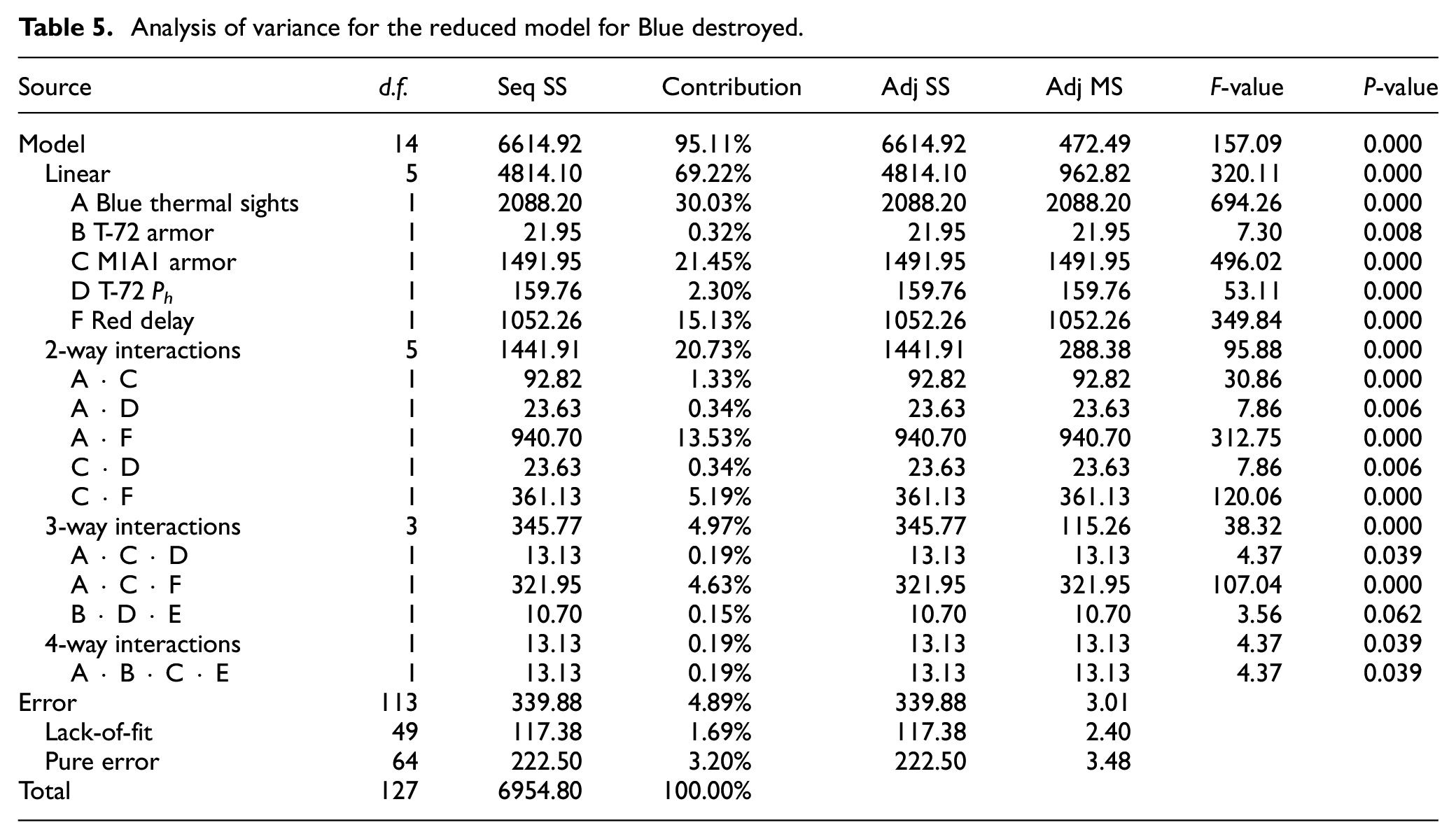
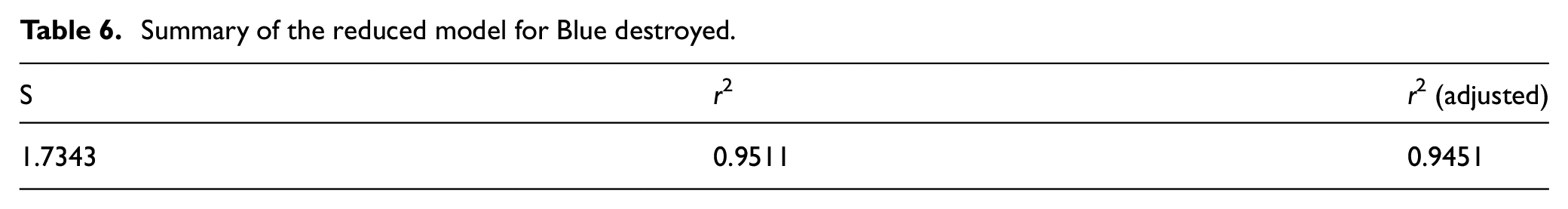
The ANOVA output in Table 5 shows that the reduced model is statistically significant, with an F-value of 157.09 and a P-value of < 0.0005. The DOE model ANOVA has an adjusted r² of 0.9451, indicating it accounts for over 90% of the variance in Blue destroyed (Table 6). All factors and interactions identified in the reduced model are statistically significant at the α = 0.05 level, except for interaction BDE (T-72 armor ċ T-72 P_hċ BMP-1 P_h), which has a P-value of 0.062. The factorial regression model for coded coefficients (Table 7) uses inputs of −1 for low factor levels and 1 for high factor levels. The regression model shows that factor A (Blue thermal sights) has by far the most substantial effect of 8.078, indicating that giving the Blue force the ability to use thermal sights decreases Blue destroyed by approximately eight vehicles. This is as expected; with thermal sights, Blue entities can identify Red entities at a range of 1600 m, while Red entities can only identify Blue vehicles visually at a range of 800 m, giving Blue a standoff distance of 800 m where Blue entities can engage Red entities without being targeted. Factor C (M1A1 armor protection), has the second largest effect of 6.828, indicating that superior M1A1 armor protection reduced Blue destroyed by approximately seven vehicles. The next most significant effects were factor F (Red delay) at 5.734 and the AF interaction (Blue thermal sights and Red delay) at 5.422.

Table 5.

Analysis of variance for the reduced model for Blue destroyed.

Source	d.f.	Seq SS	Contribution	Adj SS	Adj MS	F-value	P-value
Model	14	6614.92	95.11%	6614.92	472.49	157.09	0.000
Linear	5	4814.10	69.22%	4814.10	962.82	320.11	0.000
A Blue thermal sights	1	2088.20	30.03%	2088.20	2088.20	694.26	0.000
B T-72 armor	1	21.95	0.32%	21.95	21.95	7.30	0.008
C M1A1 armor	1	1491.95	21.45%	1491.95	1491.95	496.02	0.000
D T-72 Ph	1	159.76	2.30%	159.76	159.76	53.11	0.000
F Red delay	1	1052.26	15.13%	1052.26	1052.26	349.84	0.000
2-way interactions	5	1441.91	20.73%	1441.91	288.38	95.88	0.000
A ċ C	1	92.82	1.33%	92.82	92.82	30.86	0.000
A ċ D	1	23.63	0.34%	23.63	23.63	7.86	0.006
A ċ F	1	940.70	13.53%	940.70	940.70	312.75	0.000
C ċ D	1	23.63	0.34%	23.63	23.63	7.86	0.006
C ċ F	1	361.13	5.19%	361.13	361.13	120.06	0.000
3-way interactions	3	345.77	4.97%	345.77	115.26	38.32	0.000
A ċ C ċ D	1	13.13	0.19%	13.13	13.13	4.37	0.039
A ċ C ċ F	1	321.95	4.63%	321.95	321.95	107.04	0.000
B ċ D ċ E	1	10.70	0.15%	10.70	10.70	3.56	0.062
4-way interactions	1	13.13	0.19%	13.13	13.13	4.37	0.039
A ċ B ċ C ċ E	1	13.13	0.19%	13.13	13.13	4.37	0.039
Error	113	339.88	4.89%	339.88	3.01
Lack-of-fit	49	117.38	1.69%	117.38	2.40
Pure error	64	222.50	3.20%	222.50	3.48
Total	127	6954.80	100.00%

Table 6.

Summary of the reduced model for Blue destroyed.

S	r 2	r 2 (adjusted)
1.7343	0.9511	0.9451

Table 7.

Reduced model regression (coded coefficients) on Blue destroyed.

Term	Effect	Coef	SE coef	90% CI	T-value	P-value
Constant		7.039	0.153	(6.785, 7.293)	45.92	0.000
A Blue thermal sights	8.078	4.039	0.153	(3.785, 4.293)	26.35	0.000
B T-72 armor	0.828	0.414	0.153	(0.160, 0.668)	2.70	0.008
C M1A1 armor	6.828	3.414	0.153	(3.160, 3.668)	22.27	0.000
D T-72 Ph	2.234	1.117	0.153	(0.863, 1.371)	7.29	0.000
F Red delay	5.734	2.867	0.153	(2.613, 3.121)	18.70	0.000
A ċ C	1.703	0.852	0.153	(0.597, 1.106)	5.56	0.000
A ċ D	0.859	0.430	0.153	(0.175, 0.684)	2.80	0.006
A ċ F	5.422	2.711	0.153	(2.457, 2.965)	17.68	0.000
C ċ D	0.859	0.430	0.153	(0.175, 0.684)	2.80	0.006
C ċ F	3.359	1.680	0.153	(1.425, 1.934)	10.96	0.000
A ċ C ċ D	−0.641	−0.320	0.153	(–0.575, –0.066)	−2.09	0.039
A ċ C ċ F	3.172	1.586	0.153	(1.332, 1.840)	10.35	0.000
B ċ D ċ E	−0.578	−0.289	0.153	(–0.543, –0.035)	−1.89	0.062
Aċ B ċ C ċ E	0.641	0.320	0.153	(0.066, 0.575)	2.09	0.039

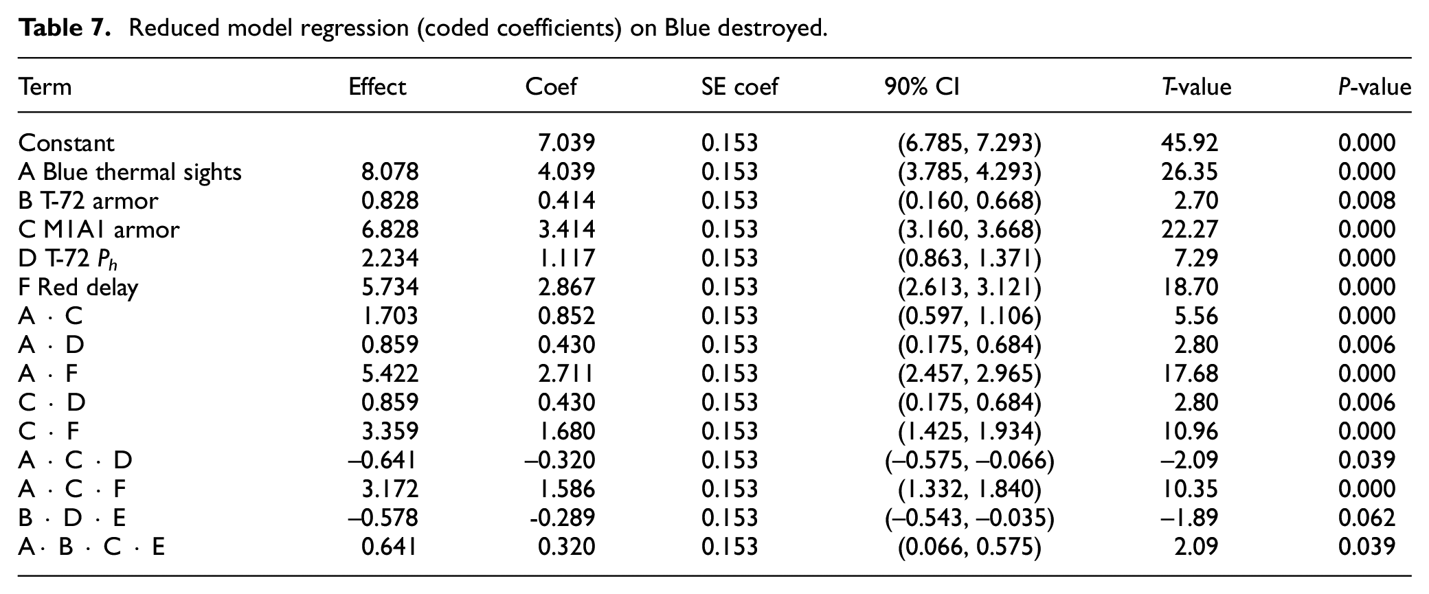
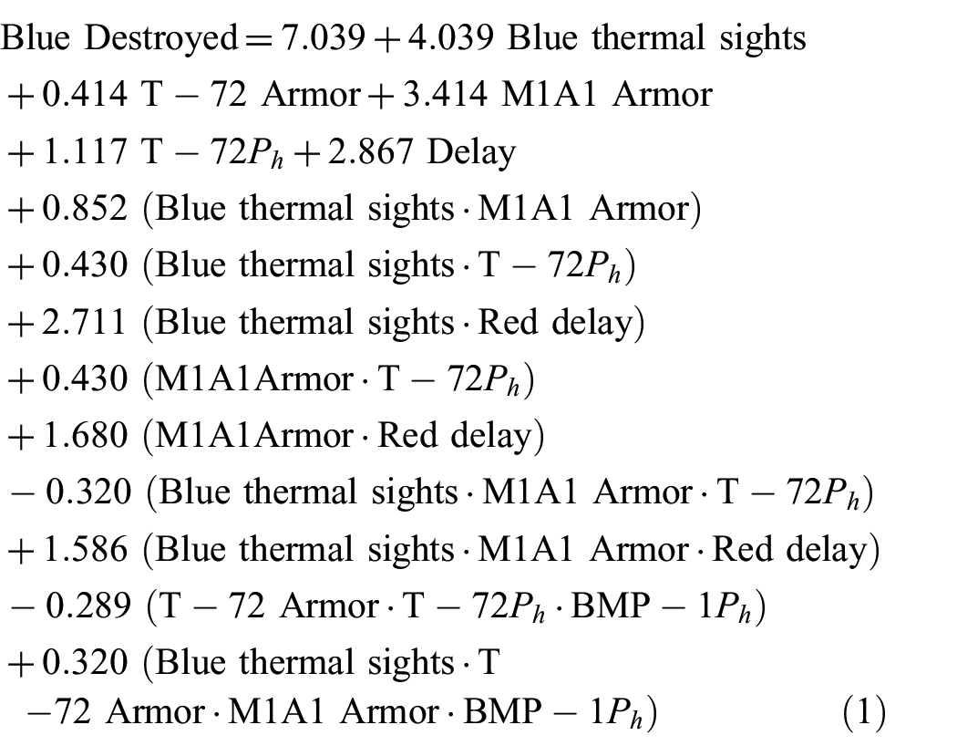
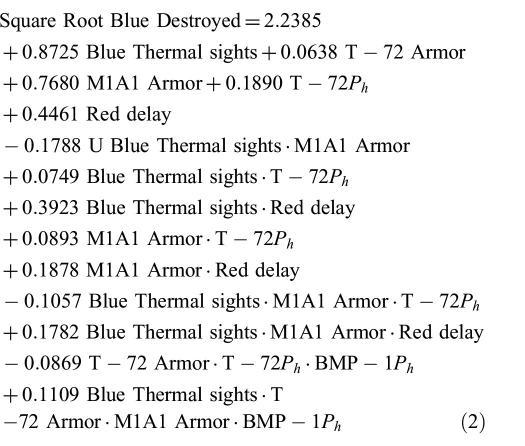
The regression equation for Blue destroyed in coded units is given by Equation (1):

$$\begin{array}{c}\mathrm{Blue}\mathrm{Destroyed}=7.039+4.039\mathrm{Blue}\mathrm{thermal}\mathrm{sights}\hfill \\ \multicolumn{1}{c}{+0.414\mathrm{T}-72\mathrm{Armor}+3.414\mathrm{M}1\mathrm{A}1\mathrm{Armor}}\\ +1.117\mathrm{T}-72P_h+2.867\mathrm{Delay}\hfill \\ \multicolumn{1}{c}{+0.852(\mathrm{Blue}\mathrm{thermal}\mathrm{sights}·\mathrm{M}1\mathrm{A}1\mathrm{Armor})}\\ +0.430(\mathrm{Blue}\mathrm{thermal}\mathrm{sights}·\mathrm{T}-72P_h)\hfill \\ \multicolumn{1}{c}{+2.711(\mathrm{Blue}\mathrm{thermal}\mathrm{sights}·\mathrm{Red}\mathrm{delay})}\\ +0.430(\mathrm{M}1\mathrm{A}1\mathrm{Armor}·\mathrm{T}-72P_h)\hfill \\ \multicolumn{1}{c}{+1.680(\mathrm{M}1\mathrm{A}1\mathrm{Armor}·\mathrm{Red}\mathrm{delay})}\\ -0.320(\mathrm{Blue}\mathrm{thermal}\mathrm{sights}·\mathrm{M}1\mathrm{A}1\mathrm{Armor}·\mathrm{T}-72P_h)\hfill \\ +1.586(\mathrm{Blue}\mathrm{thermal}\mathrm{sights}·\mathrm{M}1\mathrm{A}1\mathrm{Armor}·\mathrm{Red}\mathrm{delay})\hfill \\ -0.289(\mathrm{T}-72\mathrm{Armor}·\mathrm{T}-72P_h·\mathrm{BMP}-1P_h)\hfill \\ +0.320(\mathrm{Blue}\mathrm{thermal}\mathrm{sights}·\mathrm{T}-72\mathrm{Armor}·\mathrm{M}1\mathrm{A}1\mathrm{Armor}·\mathrm{BMP}-1P_h)\hfill \end{array}$$

(1)

4.3. Checking model assumptions

The next analyses consider whether the model is consistent with DOE assumptions. If the DOE model violates the model assumptions, additional steps are required to formulate a valid model. The DOE ANOVA model assumes that the error term in the model is normally distributed, and the error variance is constant. ²⁵ Figures 7 and 8 indicate that there is some evidence that the DOE ANOVA model may violate those assumptions. The normal probability plot (Figure 7) shows the standardized residuals versus the cumulative probability; points that fall on a line exhibit the expected cumulative probability of the normal distribution. If all of the residuals fell near the line, the distribution of the residuals would closely follow a normal distribution. The two left-most residuals are far from the line, indicating some departure from normality. The Anderson–Darling statistic is 1.122 (P-value = 0.006), indicating that the null hypothesis that the residuals are normally distributed should be rejected at the α = 0.01 significance level. The kurtosis of a normal distribution is 3, but the kurtosis of the model residuals is 2.53. For ANOVA model residual distributions with kurtosis of less than 3, the true P-value may be larger than ANOVA model calculations derived from the F-statistics, so some factors may be retained in the model that would otherwise be excluded if the correct P-values were available. ³⁸ The plot of the reduced model fitted values versus the standardized residuals for the response variable (Blue destroyed) demonstrates increasing variance in the standardized residual as the fitted values of Blue destroyed increase (Figure 8). The dispersion of the standardized residuals on the far-left side of Figure 7 is between 0 and 1, while the dispersion is between 2 and −4 on the right side of the figure, indicating that the assumption of constant variance may not be valid.

Figure 7.

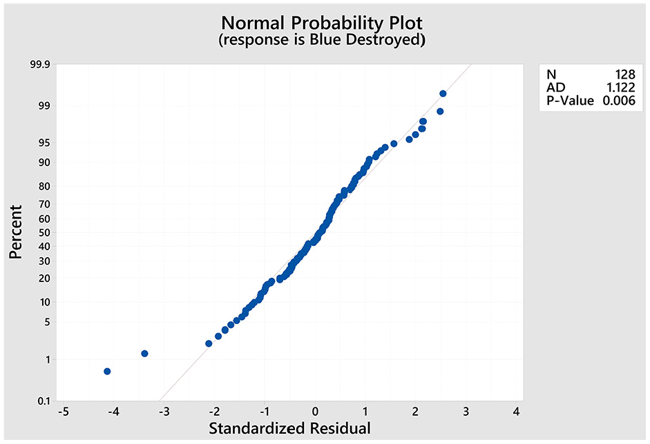
Normal probability plot of the residuals of the reduced model for response variable Blue destroyed. The plot is used to assess the ANOVA model assumption that the error term is normally distributed.

Figure 8.

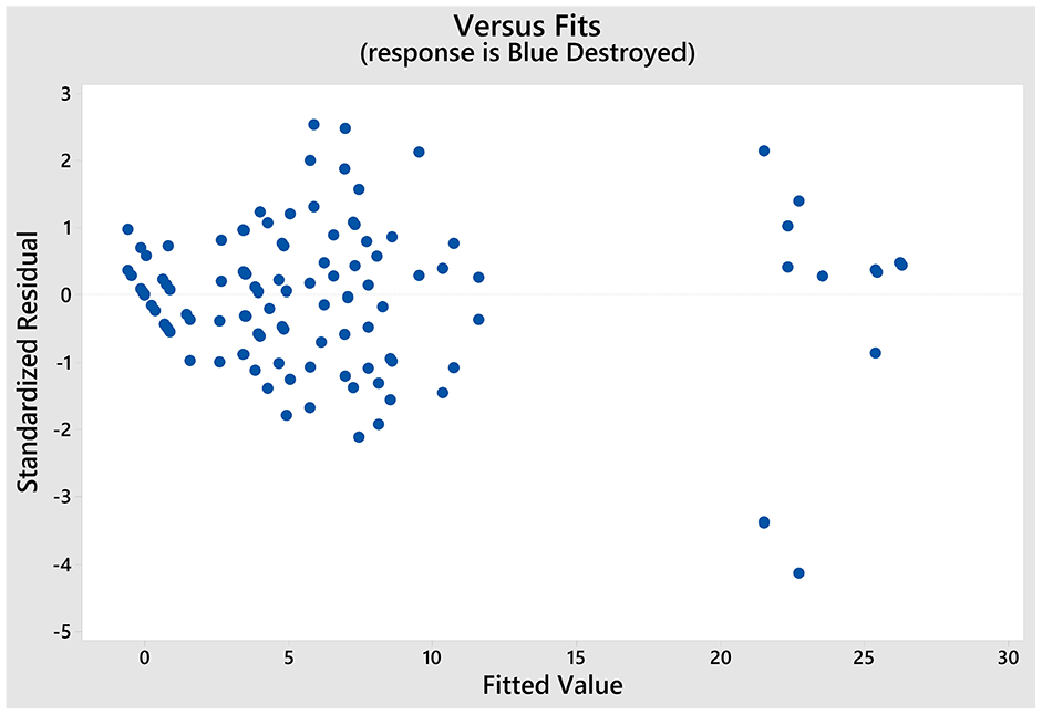
Plot of the reduced model fitted values versus the standardized residuals for the response variable Blue destroyed. The plot is used to assess the ANOVA model assumption of constant error term variance.

The model’s assumptions of normality and constant variance may not be valid, but a transformation of the response variable could result in a model that does not violate the assumptions. The response variable contained zero values, so a technique to automatically select the correct transform, the Box–Cox transform, was not feasible. ²⁵ The values that appeared to be most responsible for the violation in normality are outliers, so the model was re-run after applying a square root transform to the response variable, which reduces the impact of outliers. The assumptions of normality and constant variance appear reasonable for the DOE ANOVA model for the square root of Blue destroyed from inspection of the residual plots in Figures 9 and 10. In the normal probability plot (Figure 9), most of the standardized residuals fall near a line indicating that the residuals are close to following a normal distribution. The Anderson–Darling statistic is 0.474, with a P-value of 0.237, indicating the null hypothesis that the residuals are normally distributed cannot be rejected. The dispersion of the residuals appears relatively uniform across the values of the fitted values in the residuals versus fitted values plot (Figure 10), indicating that the assumption of constant error variance is reasonable.

Figure 9.

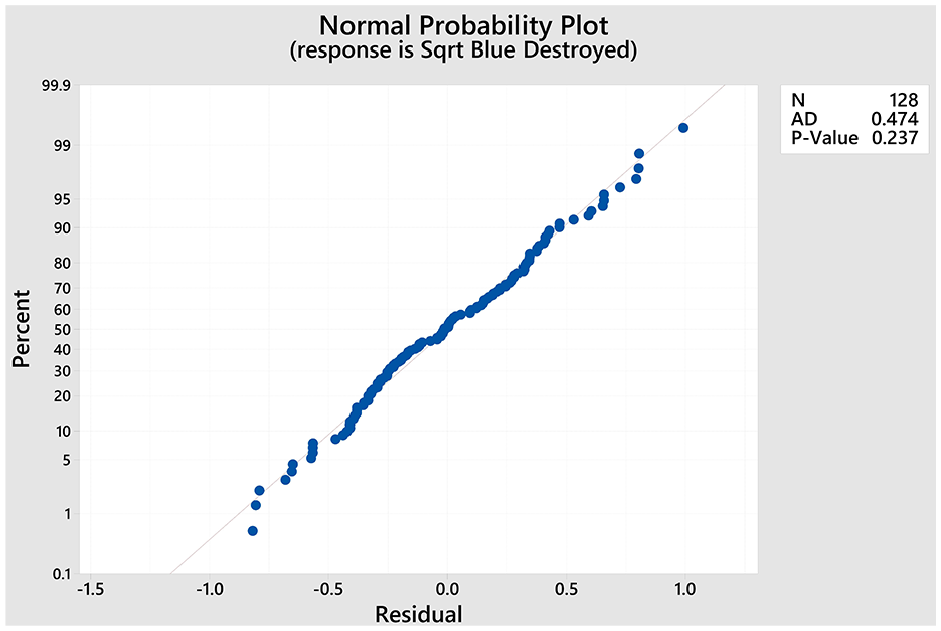
Normal probability plot of the residuals of the reduced model with the response variable square root of Blue destroyed. The plot is used to assess the ANOVA model assumption that the error term is normally distributed.

Figure 10.

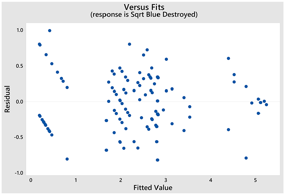
Plot of the reduced model fitted values versus the standardized residuals for the response variable square root of Blue destroyed. The plot is used to assess the ANOVA model assumption of constant error term variance.

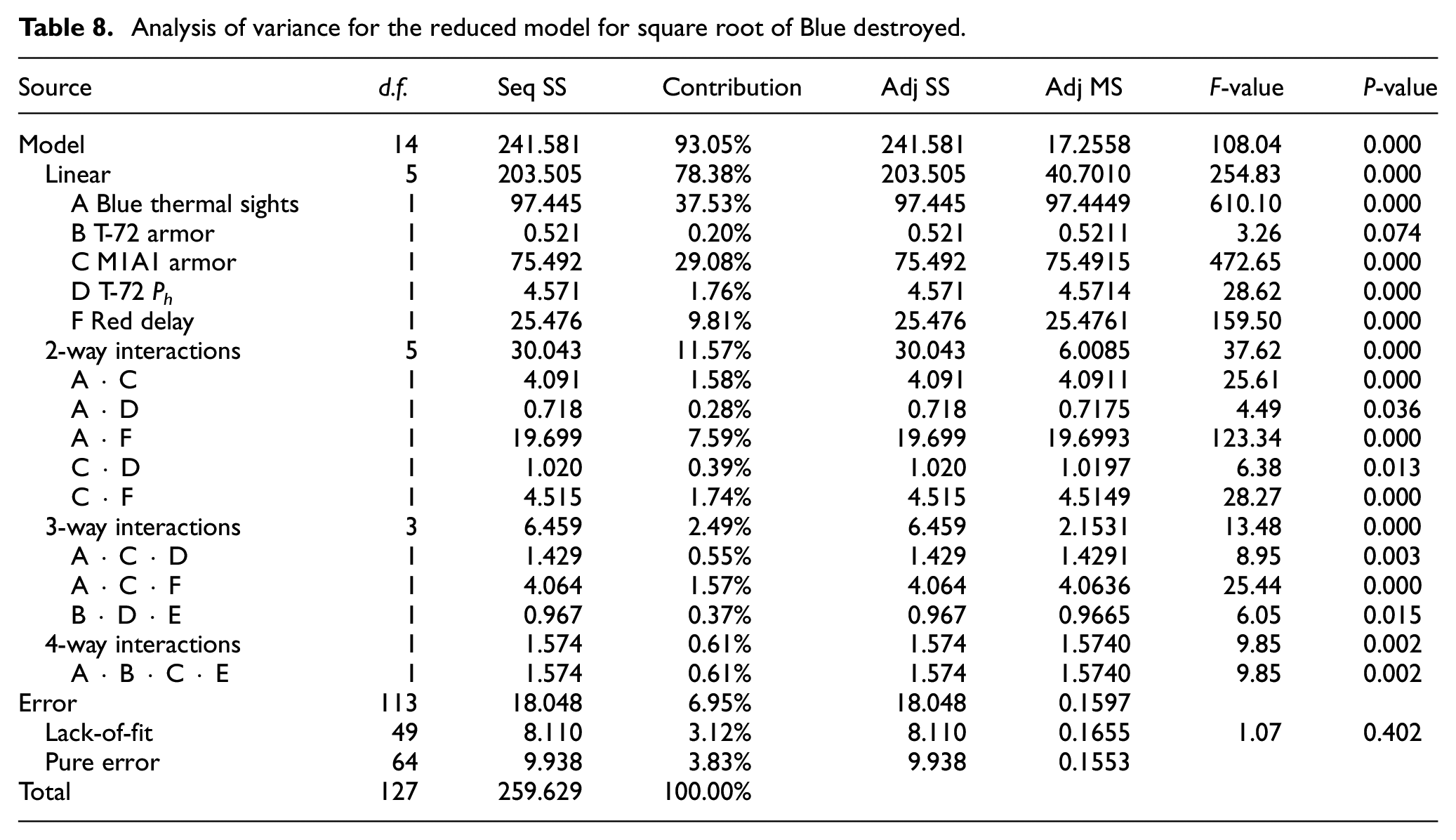
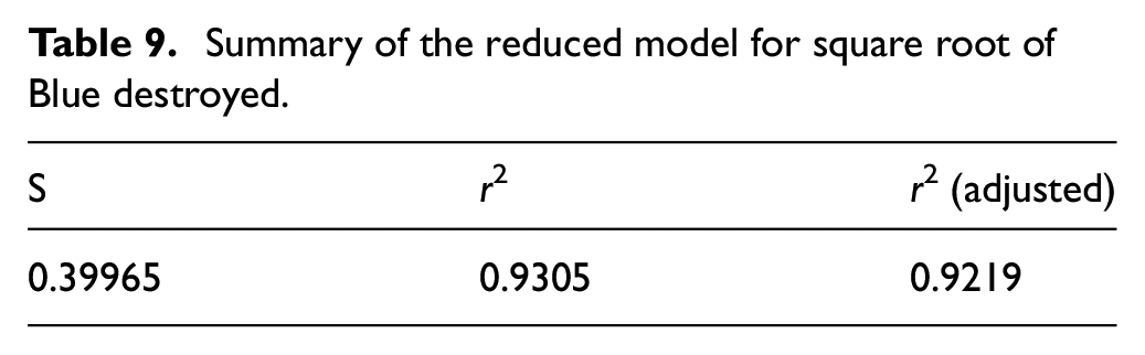
The DOE model ANOVA resulting from using the square root of Blue destroyed is different from the original reduced model before the square root transformation. In the reduced model without the transformation, all factors and interactions identified in the reduced model are statistically significant at the α = 0.05 level, except for interaction BDE (T-72 armor ċ T-72 P_hċ BMP-1 P_h). In the model with the square root transformation, several of the P-values were larger, as indicated for ANOVA residual distributions with kurtosis of less than 3. ³⁸ Notably, factor B (T-72 armor) has a P-value of 0.074 and is not significant at α = 0.05, while it was statistically significant in the original model. The interaction BDE (T-72 armor ċ T-72 P_hċ BMP-1 P_h) had a smaller P-value in the transformed model, 0.015 versus 0.062, and is therefore statistically significant at α = 0.05. The ANOVA output in Table 8 shows that the model is statistically significant, with an F-value of 108.04 and a P-value < 0.0005. The DOE model ANOVA has an adjusted r² of 0.9219, indicating the transformed model still accounts for over 90% of the variance in Blue destroyed despite being smaller than the adjusted r² for the untransformed model (Table 9).

Table 8.

Analysis of variance for the reduced model for square root of Blue destroyed.

Source	d.f.	Seq SS	Contribution	Adj SS	Adj MS	F-value	P-value
Model	14	241.581	93.05%	241.581	17.2558	108.04	0.000
Linear	5	203.505	78.38%	203.505	40.7010	254.83	0.000
A Blue thermal sights	1	97.445	37.53%	97.445	97.4449	610.10	0.000
B T-72 armor	1	0.521	0.20%	0.521	0.5211	3.26	0.074
C M1A1 armor	1	75.492	29.08%	75.492	75.4915	472.65	0.000
D T-72 Ph	1	4.571	1.76%	4.571	4.5714	28.62	0.000
F Red delay	1	25.476	9.81%	25.476	25.4761	159.50	0.000
2-way interactions	5	30.043	11.57%	30.043	6.0085	37.62	0.000
A ċ C	1	4.091	1.58%	4.091	4.0911	25.61	0.000
A ċ D	1	0.718	0.28%	0.718	0.7175	4.49	0.036
A ċ F	1	19.699	7.59%	19.699	19.6993	123.34	0.000
C ċ D	1	1.020	0.39%	1.020	1.0197	6.38	0.013
C ċ F	1	4.515	1.74%	4.515	4.5149	28.27	0.000
3-way interactions	3	6.459	2.49%	6.459	2.1531	13.48	0.000
A ċ C ċ D	1	1.429	0.55%	1.429	1.4291	8.95	0.003
A ċ C ċ F	1	4.064	1.57%	4.064	4.0636	25.44	0.000
B ċ D ċ E	1	0.967	0.37%	0.967	0.9665	6.05	0.015
4-way interactions	1	1.574	0.61%	1.574	1.5740	9.85	0.002
A ċ B ċ C ċ E	1	1.574	0.61%	1.574	1.5740	9.85	0.002
Error	113	18.048	6.95%	18.048	0.1597
Lack-of-fit	49	8.110	3.12%	8.110	0.1655	1.07	0.402
Pure error	64	9.938	3.83%	9.938	0.1553
Total	127	259.629	100.00%

Table 9.

Summary of the reduced model for square root of Blue destroyed.

S	r 2	r 2 (adjusted)
0.39965	0.9305	0.9219

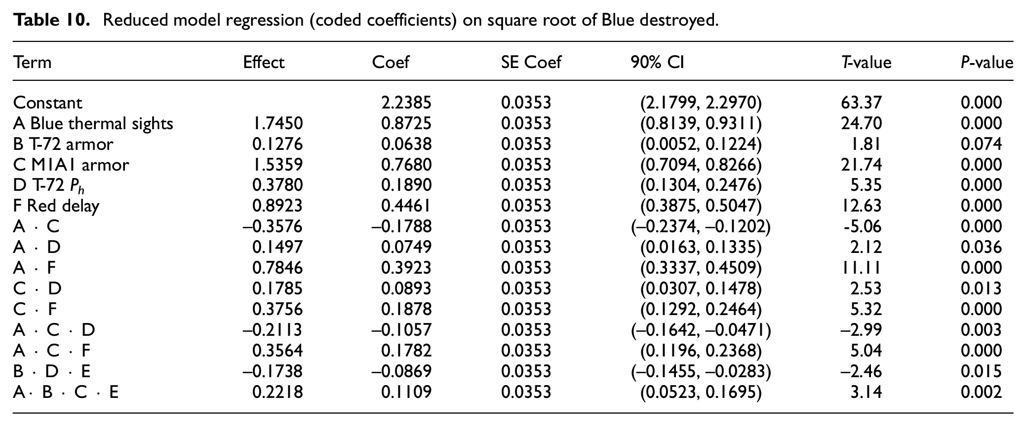
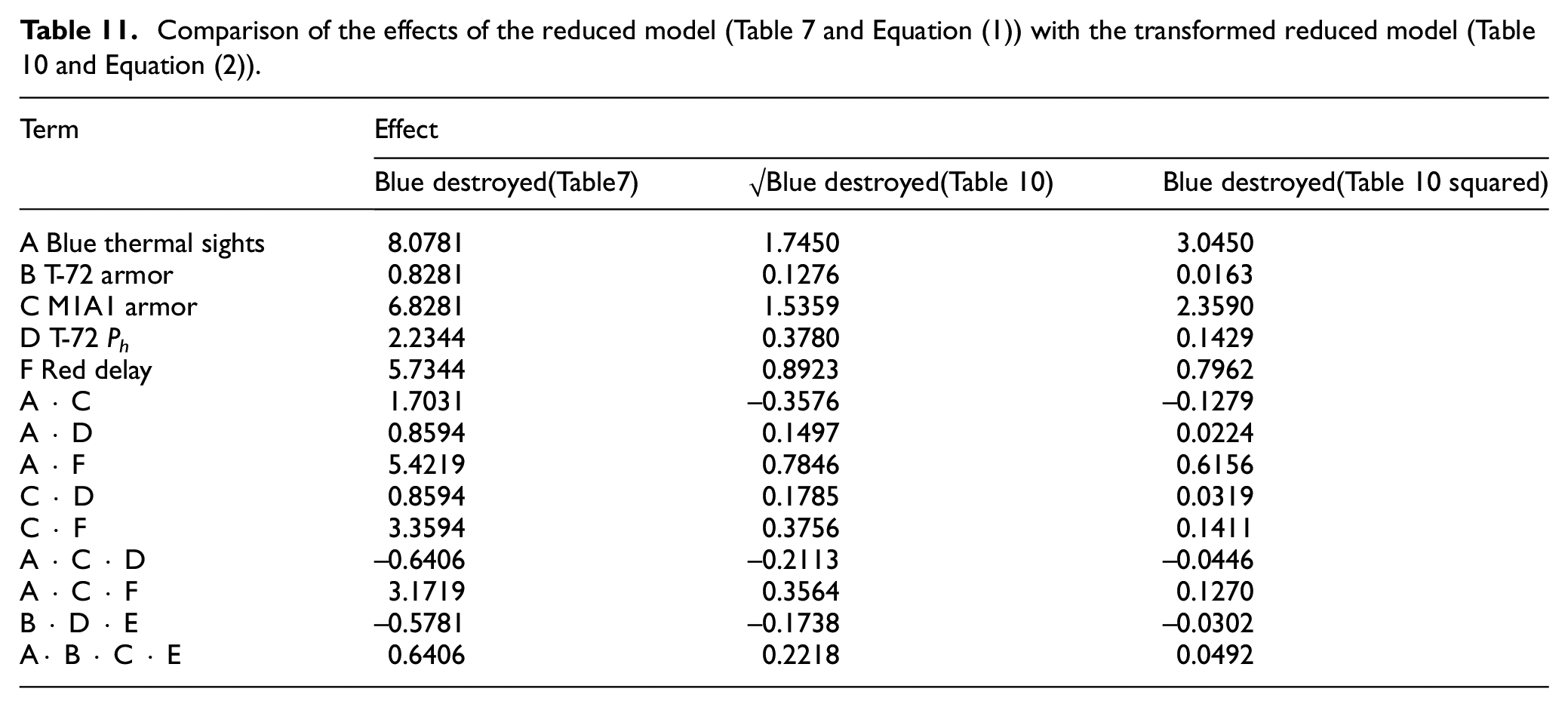
The factorial regression model for coded coefficients (Table 10) again uses inputs of −1 for low factor levels and 1 for high factor levels. Interpreting the effects of a model using the square root transformation requires squaring each effect in Table 10 to convert the units from the square root of Blue destroyed to Blue destroyed. The regression model shows that factor A (Blue thermal sights) has by far the most substantial effect of 1.7450² = 3.0464, indicating that giving the Blue force the ability to use thermal sights decreases Blue destroyed by approximately three vehicles. Again, the second most substantial effect is factor C (M1A1 armor protection) with an effect of 1.5359² = 2.3590. Table 11 displays the effects of the reduced model on Blue destroyed with the transformed reduced model. All of the effects are smaller in magnitude in the transformed model than in the untransformed model. The smaller effects in the transformed model are consistent with the hypothesis that the number of outliers in the data where the Blue forces did not have thermal sights and the Red forces had a robot swarm to provide early warning skewed the interpretation of the original model. It is also interesting that the coefficient on the AC (Blue thermal sights ċ M1A1 armor) interaction was positive in the original model, but was negative in the transformed model. This could be due to Blue’s use of thermal sights reducing the effect of the superior armor on the M1A1 tanks because the Red tanks would be destroyed before the Red tanks could target and fire on the Blue tanks.

Table 10.

Reduced model regression (coded coefficients) on square root of Blue destroyed.

Term	Effect	Coef	SE Coef	90% CI	T-value	P-value
Constant		2.2385	0.0353	(2.1799, 2.2970)	63.37	0.000
A Blue thermal sights	1.7450	0.8725	0.0353	(0.8139, 0.9311)	24.70	0.000
B T-72 armor	0.1276	0.0638	0.0353	(0.0052, 0.1224)	1.81	0.074
C M1A1 armor	1.5359	0.7680	0.0353	(0.7094, 0.8266)	21.74	0.000
D T-72 Ph	0.3780	0.1890	0.0353	(0.1304, 0.2476)	5.35	0.000
F Red delay	0.8923	0.4461	0.0353	(0.3875, 0.5047)	12.63	0.000
A ċ C	−0.3576	−0.1788	0.0353	(–0.2374, –0.1202)	−5.06	0.000
A ċ D	0.1497	0.0749	0.0353	(0.0163, 0.1335)	2.12	0.036
A ċ F	0.7846	0.3923	0.0353	(0.3337, 0.4509)	11.11	0.000
C ċ D	0.1785	0.0893	0.0353	(0.0307, 0.1478)	2.53	0.013
C ċ F	0.3756	0.1878	0.0353	(0.1292, 0.2464)	5.32	0.000
A ċ C ċ D	−0.2113	−0.1057	0.0353	(–0.1642, –0.0471)	−2.99	0.003
A ċ C ċ F	0.3564	0.1782	0.0353	(0.1196, 0.2368)	5.04	0.000
B ċ D ċ E	−0.1738	−0.0869	0.0353	(–0.1455, –0.0283)	−2.46	0.015
Aċ B ċ C ċ E	0.2218	0.1109	0.0353	(0.0523, 0.1695)	3.14	0.002

Table 11.

Comparison of the effects of the reduced model (Table 7 and Equation (1)) with the transformed reduced model (Table 10 and Equation (2)).

Term	Effect
	Blue destroyed(Table 7)	√Blue destroyed(Table 10)	Blue destroyed(Table 10 squared)
A Blue thermal sights	8.0781	1.7450	3.0450
B T-72 armor	0.8281	0.1276	0.0163
C M1A1 armor	6.8281	1.5359	2.3590
D T-72 Ph	2.2344	0.3780	0.1429
F Red delay	5.7344	0.8923	0.7962
A ċ C	1.7031	−0.3576	−0.1279
A ċ D	0.8594	0.1497	0.0224
A ċ F	5.4219	0.7846	0.6156
C ċ D	0.8594	0.1785	0.0319
C ċ F	3.3594	0.3756	0.1411
A ċ C ċ D	−0.6406	−0.2113	−0.0446
A ċ C ċ F	3.1719	0.3564	0.1270
B ċ D ċ E	−0.5781	−0.1738	−0.0302
Aċ B ċ C ċ E	0.6406	0.2218	0.0492

The regression equation for the square root of Blue destroyed in coded units is given by Equation (2):

$$\begin{array}{c}\mathrm{Square}\mathrm{Root}\mathrm{Blue}\mathrm{Destroyed}=2.2385\hfill \\ \multicolumn{1}{c}{+0.8725\mathrm{Blue}\mathrm{Thermal}\mathrm{sights}+0.0638\mathrm{T}-72\mathrm{Armor}}\\ +0.7680\mathrm{M}1\mathrm{A}1\mathrm{Armor}+0.1890\mathrm{T}-72P_h\hfill \\ \multicolumn{1}{c}{+0.4461\mathrm{Red}\mathrm{delay}}\\ -0.1788\mathrm{U}\mathrm{Blue}\mathrm{Thermal}\mathrm{sights}·\mathrm{M}1\mathrm{A}1\mathrm{Armor}\hfill \\ \multicolumn{1}{c}{+0.0749\mathrm{Blue}\mathrm{Thermal}\mathrm{sights}·\mathrm{T}-72P_h}\\ +0.3923\mathrm{Blue}\mathrm{Thermal}\mathrm{sights}·\mathrm{Red}\mathrm{delay}\hfill \\ \multicolumn{1}{c}{+0.0893\mathrm{M}1\mathrm{A}1\mathrm{Armor}·\mathrm{T}-72P_h}\\ +0.1878\mathrm{M}1\mathrm{A}1\mathrm{Armor}·\mathrm{Red}\mathrm{delay}\hfill \\ \multicolumn{1}{c}{-0.1057\mathrm{Blue}\mathrm{Thermal}\mathrm{sights}·\mathrm{M}1\mathrm{A}1\mathrm{Armor}·\mathrm{T}-72P_h}\\ +0.1782\mathrm{Blue}\mathrm{Thermal}\mathrm{sights}·\mathrm{M}1\mathrm{A}1\mathrm{Armor}·\mathrm{Red}\mathrm{delay}\hfill \\ -0.0869\mathrm{T}-72\mathrm{Armor}·\mathrm{T}-72P_h·\mathrm{BMP}-1P_h\hfill \\ +0.1109\mathrm{Blue}\mathrm{Thermal}\mathrm{sights}·\mathrm{T}-72\mathrm{Armor}·\mathrm{M}1\mathrm{A}1\mathrm{Armor}·\mathrm{BMP}-1P_h\hfill \end{array}$$

(2)

4.4. Model predictions

This section explains the predicted Blue destroyed based both on the original reduced model and the reduced model with the square root transform. Because of the possibility that the reduced model on Blue destroyed may violate critical model assumptions, estimates for the number of Blue destroyed were based on the reduced model with a square root transformation on the response. The untransformed model exhibits influence from outliers, and may violate the ANOVA assumptions of that the error term is normally distributed and has constant variance. The cube plot in Figure 11 summarizes the model predictions for the transformed reduced model from Equation (2). For later comparison, the cube plot of the predicted values for Blue destroyed using the untransformed reduced model is provided in Figure 12. The plots display predictions for all 64-factor combinations, as indicated by the labels in Figures 11 and 12. The historical evidence indicates that the Blue forces had the advantage in all six factors, so the expected coded factor combination is all six factors set to −1 or the low level. The predicted number of Blue destroyed for all factor combinations at the low level is 0.58979² = 0.3479. The actual Blue destroyed in the Eagle troop sector of the Battle of 73 Easting was zero. The predicted value of 0.3479 is closer to zero than one, so the model is reasonably calibrated at the lowest factor combination.

Figure 11.

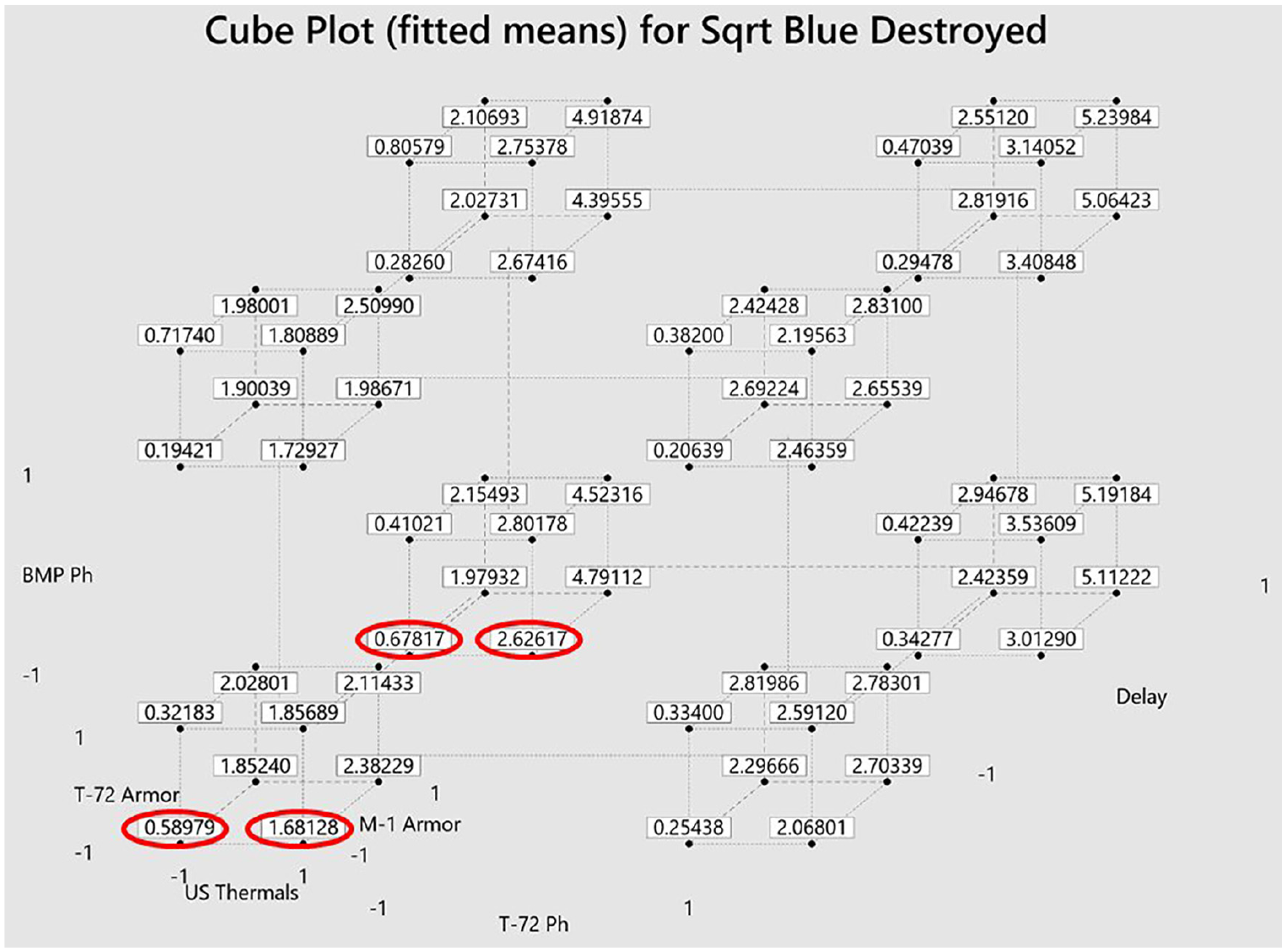
Cube plot of the transformed reduced model for the response variable square root of Blue destroyed. Each cube vertex displays the fitted value from Equation (2) for the indicated coded factor level. The square of each estimate provides the predicted number of Blue destroyed for each corresponding factor level. The circled values are the predictions for the factor combinations used in the experimental trials.

Figure 12.

Cube plot of the untransformed reduced model for the response variable Blue destroyed. Each cube vertex displays the fitted value from Equation (1) for the indicated coded factor level. The circled values are the predictions for the factor combinations used in the experimental trials.

There are several other factor combinations with Blue thermal sights where the predicted value of Blue destroyed was lower than 0.3479. The number of Blue destroyed for both replicates with the combination where all six factors were set to the low level was one Blue vehicle destroyed. Many other combinations of factors that included Blue thermal sights recorded zero Blue vehicles destroyed. Given that any factor level at the high level provides some advantage to the Red forces, it is likely that a DOE model with more replicates would have produced estimates where the combination of all low factors had the smallest estimate of Blue destroyed.

The baseline model for the estimate of the effect of a robot swarm on the outcome of the model is, therefore, the case where all six factor levels are at the low level. The effect of adding the robot swarm to increase Red for situational awareness is modeled with the factor combination of all factors at the low level (–1 in coded units) while the Red delay factor is at the high level (1 in coded units). The estimate recorded in Figure 11 is 0.67817² = 0.4599. The predicted effect of adding the robot swarm is therefore minimal: 0.4699 – 0.3479 = 0.1220. The result is due to the strong interaction between factor F (Red delay) and the two factors with the largest effects, factor A (Blue thermal sights) and factor C (M1A1 armor protection). At the low level of factor A, Blue vehicle crews can identify and engage Red vehicles at 1600 m, while Red forces cannot effectively engage Blue vehicles until the distance between the forces is 800 m. Factor C (M1A1 armor) and F (Red delay) are made mostly irrelevant by the thermal sights because many of the Red vehicles would be destroyed before they could identify Blue vehicles approaching even if the Red crews were ready to fight. Similarly, Red forces cannot test the M1A1 armor protection regardless of the level of factor C if they cannot identify the approach of the Blue force. With factor A set to the high level (no Blue thermal sights), the predicted number of Blue destroyed with a robot swarm present, i.e., factor F at the high level (no Red delay), is 2.62617² = 6.8968 versus 1.68128² = 2.8267 without a robot swarm supporting Red. The predicted effect of the robot swarm is 6.8968 – 2.8267 = 4.0701 or about four additional Blue destroyed.

5. Robot swarm experiments

The effect of a robot swarm is estimated using the calibrated model both with and without the dominating effect of factor A (Blue thermal sights) in this section. The results of experimental runs of 30 trials of each of four different factor combinations using the calibrated model are reported. Additionally, the results of the trials are used to recommend refinements to the calibration model.

5.1. Effect of the robot swarm

This section assesses the potential impact of a robot swarm to increase situational awareness using the extra statistical power of additional trials of the calibrated model focused on specific factor combinations. The calibrated model was used to conduct four experiments each consisting of 30 trials (executions of the 73 Easting scenario), for a total of 120 additional model runs. The effect of employing a robot swarm to eliminate the delay in Red response to a Blue attack was estimated by comparing the results of the trials. The DOE model had only two replicates at each factor level, so repeating the experiments 30 times at each factor level improved the power of each estimate.

Indeed, for the historical baseline case where the Blue forces had the advantage in all six factor levels, both replicates of the DOE model resulted in outcomes with one Blue vehicle destroyed in each trial. Over the 30 trials in the experimental runs where all six factor levels were set to the low level, 25 of the 30 trials resulted in zero Blue force vehicles destroyed.

The remaining five trials resulted in one Blue vehicle destroyed in each trial. Through random selection, both DOE replicates resulted in an outcome that occurred in only 1/6 of the experimental runs, which accounts for higher estimated losses in the baseline case as compared with similar factor combinations with one of the other factors (B, D, or E) with small effects also set to the high level.

Table 12 and Figure 13 show the estimate of the effect of a robot swarm on the Battle of 73 Easting, comparing the base case where all six factors favored Blue forces to the case where the robot swarm eliminated the delay in Red force reaction. In both cases, the Blue forces were able to use thermal sights. The average number of Blue vehicles destroyed in trials where the Red forces used a robot swarm was 0.267, whereas in those trials with no Red robot swarm and consequently a delay in Red reaction, the average number of Blue destroyed was 0.167. The addition of the robot swarm to prevent the Red delay increased Blue destroyed by only 0.100. The difference in the means of the two sets of trials was not statistically significant at the α = 0.05 level with a P-value of 0.399. The results are consistent with the small difference predicted by the DOE model of 0.1220, with both estimates indicating that a robot swarm would have had little or no effect on the outcome of the historical battle.

Table 12.

Statistical comparison of the effects of Red delay and no Red delay when the Blue force had thermal sights. Factors B, C, D, and E were set to the low level all for trials.

Trial type	n	Mean	Std dev	SE mean
Blue thermal sights/no Red delay (μ1)	30	0.267	0.521	0.095
Blue thermal sights/Red delay (µ2)	30	0.167	0.379	0.069
Null hypothesis	H 0: μ1–µ2 = 0
Alternative hypothesis	H 1: μ1–µ2≠ 0
Difference μ1–µ2	95% CIfor difference	T-value	d.f.	P-value
0.100	(–0.136, 0.336)	0.85	52	0.399

Figure 13.

Box plot comparing the effects of Red delay and no Red delay when the Blue force had thermal sights. Factors B, C, D, and E were set to the low level for all trials. Diamonds indicate outliers.

The experimental results support the conclusion from the DOE model that a strong interaction between factors A and F reduces the effect of the Red robot swarm when the Blue forces have thermal sights. In other words, the disadvantage of poor situational awareness is mostly irrelevant due to the capabilities of the thermal sights. Table 13 and Figure 14 show the results comparing the effect of the robot swarm when the Blue forces are denied the use of thermal sights. If Blue does not have thermal sights, the average number of Blue vehicles destroyed in trials with a Red robot swarm was 7.333, whereas in those trials with no Red robot swarm the average number of Blue destroyed was 2.533. In the absence of Blue thermal sights, the addition of the robot swarm to eliminate the Red delay increased Blue destroyed by 4.800. The difference in the means of the two sets of trials was statistically significant at the α = 0.05 level with a P-value of < 0.0005. Importantly, note that the increases in Blue destroyed by the DOE model (4.0701) and estimated by the experimental runs of the calibrated combat model (4.800) are quite consistent.

Table 13.

Statistical comparison of the effects of Red delay and no Red delay when the Blue force did not have thermal sights. Factors B, C, D, and E were set to the low level for all trials.

Trial type	n	Mean	Std dev	SE mean
No Blue thermal sights/No Red delay (μ1)	30	7.33	1.86	0.34
No Blue thermal sights/Red delay (µ2)	30	2.53	1.48	0.27
Null hypothesis	H 0: μ1–µ2 = 0
Alternative hypothesis	H 1: μ1–µ2≠ 0
Difference μ1–µ2	95% CIfor difference	T-value	d.f.	P-value
4.800	(5.670, 3.930)	11.05	55	0.000

Figure 14.

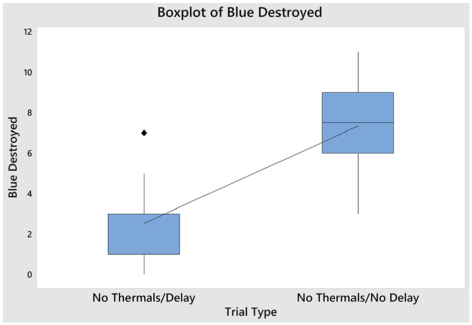
Box plot comparing the effects of Red delay and no Red delay when the Blue force did not have thermal sights. Factors B, C, D, and E were set to the low level for all trials. Diamonds indicate outliers.

A previous analysis of the Battle of 73 Easting, which used a regression model, included tactical employment factors not considered in this study, such as whether or not the Red tanks were properly dug in. ³⁴ By assuming the use of human scouts to provide an early warning to the Red forces, that study estimated that the historical delay in Red reaction reduced Blue destroyed by approximately 1.80. The earlier analysis also noted a strong interaction between the Blue use of thermal sights and the Red delay due to a lack of early warning. ³⁴ While the earlier estimate is lower than the estimate in the current study, the small magnitude of the direct effect and the strong interactions are consistent with the current study’s results.

5.2. Assessment of the DOE model calibration

The purpose of this section is to assess the estimates of the DOE model for combinations of the most significant factors using additional simulation trials. The DOE estimates were designed to produce estimates using the minimum number of trials to achieve the desired statistical power, which was two replicates at each factor combination according the power analysis in Section 3.4. This section evaluates the accuracy of the estimates using additional trials for combinations of the factors with the largest estimated effects.

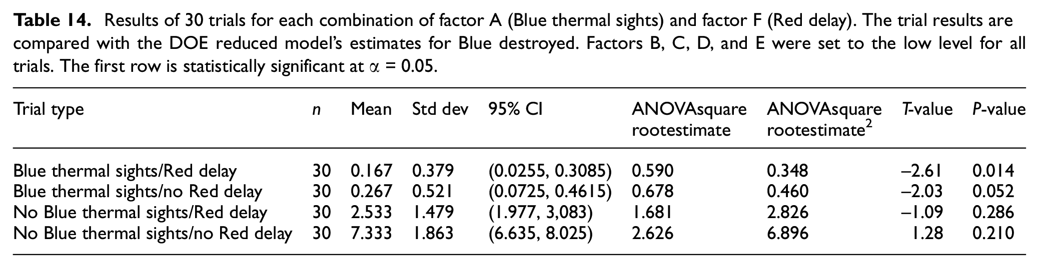
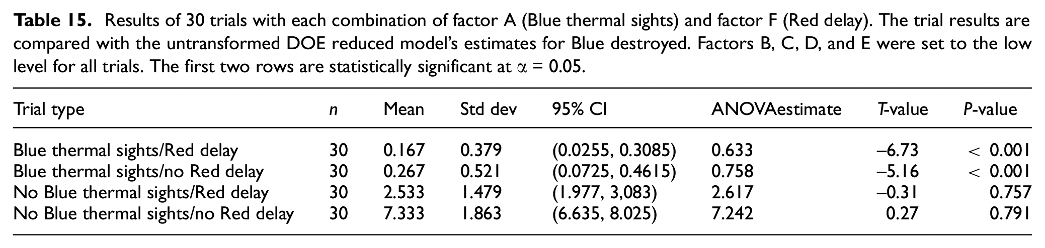
A comparison of the DOE model predictions with the results of the experimental trials indicates that the DOE model did not accurately predict the experimental results for the factor combinations where Blue forces used thermal sights. Tables 14 and 15 list a comparison of the DOE ANOVA estimates for the square root of Blue destroyed, and the untransformed Blue destroyed models, respectively, with the experimental results. The P-values in the table report the results of a t-test with null hypothesis H₀: μ = ANOVA estimate and alternative hypothesis H₁: μ≠ ANOVA estimate. All of the ANOVA estimates for factor combinations that included Blue thermal sights were substantially higher than the corresponding results of the experimental trials. Three of the four estimates for factor combinations with thermal sights in Tables 14 and 15 had a statistically significant difference from the respective experimental mean. A reasonable estimate of the mean should fall in the confidence interval for the experimental mean. The DOE ANOVA estimates are likely biased by the outliers depicted in the box plot in Figure 5. The box plot shows 14 outliers; all of the outliers are factor combinations that do not include Blue thermal sights and do include a Red robot swarm. All of the estimates for combinations that do not include Blue thermal sights are in the confidence interval around the experimental mean and are not statistically different from the experimental mean. The factor combinations that did not include Blue thermal sights produced estimates that were closer in value to the outliers and were, therefore, less susceptible to bias.

Table 14.

Results of 30 trials for each combination of factor A (Blue thermal sights) and factor F (Red delay). The trial results are compared with the DOE reduced model’s estimates for Blue destroyed. Factors B, C, D, and E were set to the low level for all trials. The first row is statistically significant at α = 0.05.

Trial type	n	Mean	Std dev	95% CI	ANOVAsquare rootestimate	ANOVAsquare rootestimate 2	T-value	P-value
Blue thermal sights/Red delay	30	0.167	0.379	(0.0255, 0.3085)	0.590	0.348	−2.61	0.014
Blue thermal sights/no Red delay	30	0.267	0.521	(0.0725, 0.4615)	0.678	0.460	−2.03	0.052
No Blue thermal sights/Red delay	30	2.533	1.479	(1.977, 3,083)	1.681	2.826	−1.09	0.286
No Blue thermal sights/no Red delay	30	7.333	1.863	(6.635, 8.025)	2.626	6.896	1.28	0.210

Table 15.

Results of 30 trials with each combination of factor A (Blue thermal sights) and factor F (Red delay). The trial results are compared with the untransformed DOE reduced model’s estimates for Blue destroyed. Factors B, C, D, and E were set to the low level for all trials. The first two rows are statistically significant at α = 0.05.

Trial type	n	Mean	Std dev	95% CI	ANOVAestimate	T-value	P-value
Blue thermal sights/Red delay	30	0.167	0.379	(0.0255, 0.3085)	0.633	−6.73	< 0.001
Blue thermal sights/no Red delay	30	0.267	0.521	(0.0725, 0.4615)	0.758	−5.16	< 0.001
No Blue thermal sights/Red delay	30	2.533	1.479	(1.977, 3,083)	2.617	−0.31	0.757
No Blue thermal sights/no Red delay	30	7.333	1.863	(6.635, 8.025)	7.242	0.27	0.791

One possible reason for a large number of outliers is the values used to define the factor levels may have been unrealistically high or low. The amount of time for the Red delay was not specified in the historical record; consequently, the value used in this study was based on subject matter expert estimates. The DOE model could be expanded with some center points to test for curvature and examine different time delays. Factor C (M1A1 armor) could also have values that are unrealistically low. The evidence in the historical record documenting the effective range of both the thermal and optical-visual sights was based on the estimates of actual participants in the battle, so adjusting factor A would require more caution. ³² Future work could include fine-tuning factor levels to produce a DOE ANOVA model that better meets the model assumptions and produces better estimates when compared with the experimental runs.

6. Conclusions, contributions, and future work

The DOE ANOVA model used to calibrate the simulation model and the 30 trials for each of four combinations of two factor levels show that the effect of employing robot swarms to improve early warning is not linear, but instead depends on other military technologies and the tactics the opposing forces might use. For the historical Battle of 73 Easting, where the Blue forces had thermal sights, the estimated effect of a robot swarm was not statistically significant and a robot swarm is therefore considered unlikely to have had an impact on the outcome of the historical battle. The advantage provided by the thermal sights—the Blue forces could target the Red forces before Red could target Blue—overwhelmed the benefit of a notional robot swarm. The effect of the robot swarm had strong interactive effects with both the Blue thermal sights and M1A1 armor protection. However, in trials where both forces had the same targeting ability, the effect of the robot swarm was more substantial and statistically significant and potentially could have had a significant effect on the outcome of the battle.

The study provides two contributions: (1) an initial estimate of the impact of a robot swarm, and how that impact can be linked to the availability of other technologies, and (2) a demonstration or example of how to use rigorous DOE methods to improve the reliability of results obtained using SAF systems.

The ongoing proliferation of advanced military technology suggests that it is less likely that any future force would enjoy as many advantages as the Blue forces did in the Gulf War. Future battles with robot swarm employment will likely be between more equally matched forces where the interaction between other technologies, and robot swarm capabilities and tactics, could be important or even decisive. The strong interactions between robot swarm employment and other factors on the battlefield will likely motivate the use of constructive entity-level combat models to develop robotic systems and tactics to employ them. Future studies should explicitly include tactics for the robot swarms and any different tactics for the human members of a force.

The DOE model calibration methodology provides a useful tool for exploring the contribution of various factors and interactions to the effects estimated by a constructive entity-based model. Understanding the relative contributions of the various factors and the interactions between factors can help in interpreting the results, as well as aiding the verification and validation process. Future studies should include using center points or response-surface methodologies to fine-tune factor-level parameter settings in cases where the initial model exhibits potential violations of the statistical assumptions and the presence of outliers.