Avoiding the eyeballing fallacy: Visualizing statistical differences between estimates using the pheatplot command

Abstract

Graphical representations of coefficients and their confidence intervals are increasingly used in research presentations and publications because they are easier and quicker to read than tables. However, in coefficient plots that include several estimated coefficients, researchers often use confidence intervals to eyeball whether coefficients are statistically significant from each other, which results in an overly conservative test and increased risk of type II errors. To help avoid this eyeballing fallacy, we introduce the pheatplot postestimation command, which visualizes the statistical significance across estimates of categorical variables in a regression model. pheatplot efficiently compares the significance level between point estimates and helps researchers avoid making wrong assumptions about whether estimates differ. Moreover, by representing $p$ -values as continuous measures rather than binary thresholds, it provides the flexibility to move beyond arbitrary cutoffs of statistical significance. This article offers some examples that illustrate the functionality of the pheatplot command.

1 Introduction

Graphical presentation of coefficients and confidence intervals (CIs) of regression results are increasingly used in research presentations and publications because they are easier and quicker to read than tables. So-called coefficient plots facilitate an immediate and highly accessible understanding of the estimates’ relative sizes and their precision. Moreover, if a $95\text{\%}$ CI of an estimate overlaps with 0, there is no statistically significant difference between the estimate of its given size and 0, given the conventional criterion of significance set to an alpha level of 0.05. This way, coefficient plots can be efficiently used to infer whether estimates differ significantly from zero.

However, in coefficient plots that include several estimates, researchers often use the CIs to eyeball whether coefficients differ significantly from each other and not only if they are significantly different from zero. For example, with categorical variables included as a set of indicator variables, researchers often want to assess whether there is a statistically significant difference between pairwise estimates. Comparing whether CIs of separate coefficients overlap is a frequent approach. However, while it is tempting to use the CIs in this way, such inference is wrong in many cases (Belia et al. 2005) For example, while there is always a statistically significant difference at the $5\text{\%}$ level between $95\text{\%}$ CIs that do not overlap, it is well known that the difference might be statistically significant despite overlapping CIs (Belia et al. 2005; Schenker and Gentleman 2001; Payton, Greenstone, and Schenker 2003; Greenland et al. 2016). Thus, eyeballing whether CIs overlap increases the likelihood of type II errors.

To ease the comparison of coefficients from a linear regression model, we provide the postestimation command pheatplot, which can be used after various regression models to visually represent statistical differences in estimates between values of categorical variables or differences in effects of an interaction variable by values of a categorical variable. When dealing with a small number of categories, we can conduct pairwise comparisons effectively through manual statistical tests or by displaying the CIs of the differences between estimates (for example, Goisis et al. [2023]). However, as the number of categories to be compared grows, manually comparing regression coefficients is both tedious to perform and challenging to present. For instance, when we compare 3 categories, there are 3 possible pairwise comparisons, while as the number of categories increases to 5, the number of pairwise comparisons grows to 10. The pheatplot postestimation command allows the user to visualize statistical significance compactly by using heat plots (Jann 2019) to visualize the $p$ -values of pairwise tests. This way, pheatplot offers an efficient visualization of the significance level of the differences between point estimates and helps avoid making wrong assumptions about whether estimates differ.

Moreover, the pheatplot command provides the flexibility to move beyond the traditional $p<0.05$ significance threshold, aligning with recent discussions in the statistical community, exemplified by editorials in publications like American Statistician (Wasserstein, Schirm, and Lazar 2019), Nature (Nature 2019), and Demographic Research (Bijak 2019). While it is widely acknowledged that drawing conclusions based solely on discrete $p$ -value thresholds is not advisable, the caution against using $p$ -values as arbitrary indicators of significance is often unheeded. By representing $p$ -values as continuous measures rather than binary thresholds, pheatplot addresses these concerns. It encourages a more nuanced and informative interpretation of the statistical significance of the differences between estimates rather than simply labeling them as significant or not based on arbitrary cutoffs.

Finally, pheatplot minimizes coding requirements, saving time and reducing the chance of coding errors, thus fostering transparency and replicability. It is most convenient for examining pairwise comparisons when the number of categories is between 4 and 20 (that is, between 6 and 190 pairwise comparisons).

In the following, we begin with a brief description of what we call the eyeballing fallacy and provide an example of how to use a heat plot to visualize differences in significance between coefficients. Then we introduce the pheatplot command, along with some examples of use, before we give a brief conclusion.

2 The eyeballing fallacy of overlapping CIs

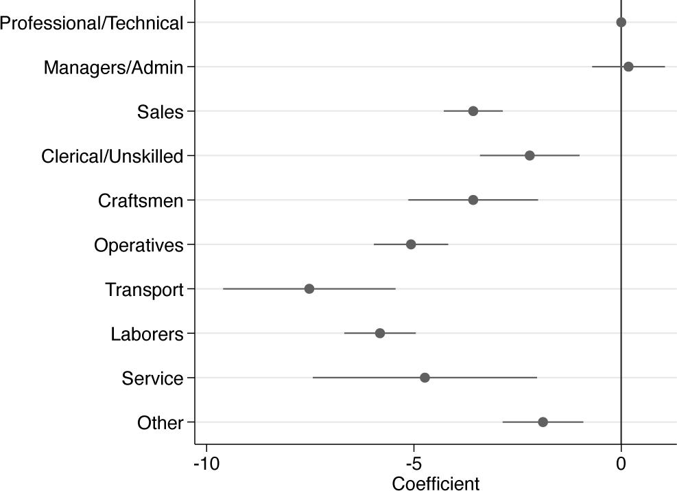
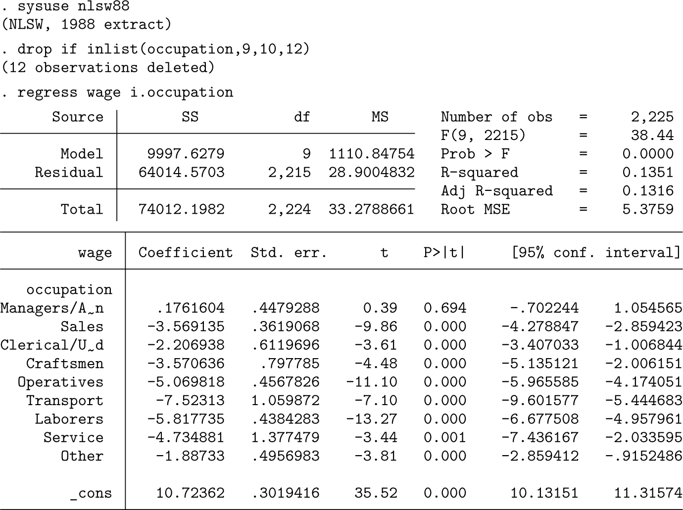
To demonstrate the potential fallacy of eyeballing CIs to infer whether differences between coefficients are statistically significant, let us consider a practical example. As an illustration, we use a subsample of the National Longitudinal Survey (nlsw88.dta) containing data from a group of women in their 30  s or early 40  s to investigate differences in hourly wages between occupations. We conduct a linear regression analysis and use the coefplot command (Jann 2014) to visualize occupation coefficients and their respective $95\text{\%}$ CIs, setting workers with professional occupations as the reference category (figure 1).

Figure 1.

Coefficient plot of occupation indicators

Upon examining the estimates and CIs, we can easily conclude whether the various occupations differ relative to professionals, the reference category, by checking whether the CIs overlap with zero. Based on the coefficient plot in figure 1, we can conclude that managers and administrators have statistically indistinguishable hourly wages compared with professionals, while workers in all other occupations exhibit lower hourly wages.

However, what about wage differences between the other occupations? When CIs are nonoverlapping, we can infer that there is a significant hourly wage difference at the $5\text{\%}$ level (or other levels, depending on the calculation of the CIs). For example, there is a significant difference between clerical or unskilled workers and operatives. In contrast, when CIs overlap, we cannot easily conclude whether wage differences are statistically significantly different at the $5\text{\%}$ level. For example, the CIs for the coefficient of clerical or unskilled workers overlap with those of both craftsmen and sales occupations. Yet while a t test that compares coefficients of clerical or unskilled workers against craftsmen yields a $p$ -value of 0.134, supporting the null hypothesis, the $p$ -value of the difference between clerical or unskilled workers and sales workers is 0.017, indicating strong enough evidence to reject the null hypothesis.

The eyeballing fallacy of comparing CIs of two coefficients has long been discussed (for example, Cole and Blair [1999]; Schenker and Gentleman [2001]; Austin and Hux [2002]; Knol, Pestman, and Grobbee [2011]). Some have suggested adjusting calculations of the coefficients’ CIs so that they do not overlap when the estimates are significantly different from each other at a chosen confidence level (for example, Cumming and Finch [2005]; Goldstein and Healy [1995]). However, this would demand communication from the writer to clarify for the reader that the CIs are to be interpreted differently from what one usually expects. Others have calculated approximations or rules of thumb of how much CIs can overlap for estimates that are, in reality, significantly different, such as Cumming (2009) and Afshartous and Preston (2010). However useful, this would probably not alleviate the writer from explaining in text which estimates are different from each other and which are not. Others, again, suggest visualizing CIs with gradations (Kohler and Eckman 2011). While this has the benefit of highlighting that the parameter estimate is more likely to lie near the center of the interval than at its endpoints, it can still be hard to draw conclusions on whether two groups differ. Finally, some propose not to use the CIs of the estimates as a reference point but rather to visualize the significance level of the difference itself (Goisis et al. 2023). However, when the number of coefficients is large—and we want to avoid relying on an arbitrary cutoff of what is deemed statistically significant and what is not—it is challenging to convey the results in a way that does not gravely complicate visualization and demands extensive explanations.

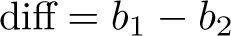
To ease the comparison of coefficients from a linear regression model, we suggest visually representing the estimates’ statistical difference using a heat plot. Although the logic applies to all regression coefficients, we will focus the discussion (and the pheatplot command, introduced below) on categorical variables. Let $b_1$ and $b_2$ be two estimated regression coefficients that we want to compare, such as the wages of clerical workers $(b_1)$ and workers within sales ( $b_2$ ) compared with the reference group professional workers. The differences between coefficients from a single regression mode. are calculated as

$$\mathrm{diff}=b_1-b_2$$

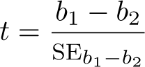
and the standard error (SE)of the differences as

$${\mathrm{SE}}_{b_1-b_2}=\sqrt{\mathrm{Var}(b_1)+\mathrm{Var}(b_2)-2\mathrm{Cov}(b_1,b_2)}$$

Using the difference and the SE of the difference, we can calculate the $t$ -value and then get the p-value.

$$t={\displaystyle \frac{b_1-b_2}{{\mathrm{SE}}_{b_1-b_2}}}$$

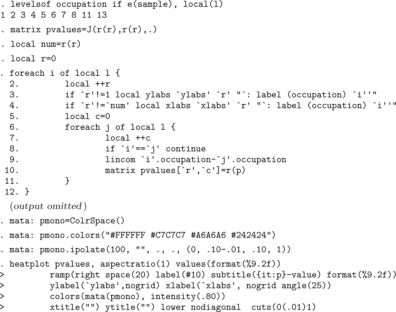
In Stata, we can calculate such pairwise comparisons using lincom. Moreover, we can loop over the values of our categorical occupation variable and store all pairwise comparisons in a matrix before plotting them using the community-contributed command heatplot (figure 2).

Figure 2.

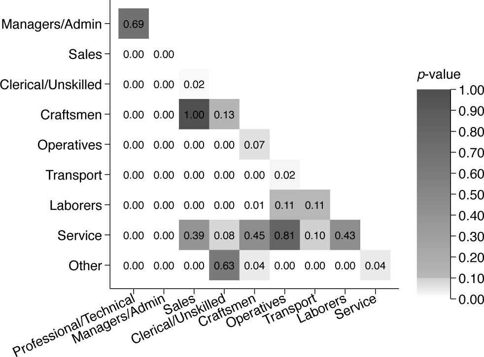
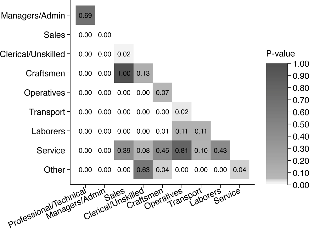
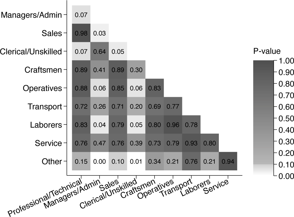
Heat plot of $p$ -values of the difference between model coefficients

Based on this heat plot, it is easy to gauge the statistical significance of the difference between the various coefficients. We can see that most of the pairwise comparisons are statistically significant at the $5\text{\%}$ level but also how they differ around the arbitrary $5\text{\%}$ level, as indicated by the white and lighter grayscale. Furthermore, the cell numbers provide the $p$ -values. For example, we see that the $p$ -value of the difference between craftsmen and clerical or unskilled workers is 0.13, while the corresponding $p$ -value of the difference between sales and clerical or unskilled workers is 0.02. The pheatplot command, introduced in the following section, automates the creation of such graphs.

3 The pheatplot command

pheatplot is a postestimation command that calculates pairwise comparisons of estimates using lincom and provides a heat plot by color to visualize the $p$ -values of the difference between the categories of a factor variable or their interaction effects. It can be used after all single-equation estimation commands that allow for factor-variable notation and the use of the postestimation command lincom. In the pheatplot syntax, the categorical variable to be compared is placed after the command name, followed by options.

3.1 Syntax

pheatplot varname [, threshold(#) interaction(varname)

frame(newframename) pname(name) bname(name) heatoptsp(options)

heatoptsb(options) pvalues(off) savetable(filename[, save_options])

savegraph(filename.suffix[, replace]) hexplot differences mono]

3.2 Options

threshold(#) sets the critical threshold value, with the color gradient differing below and above this threshold. This allows the user to identify and communicate whether differences are statistically significant at specific levels while simultaneously avoiding strict cutoff values. The default is threshold(.10).

interaction(varname) specifies the interaction variable, if any. Interactions must be included using factor-variable operators (he1p fvvarlist).

frame(newframename) specifies the name of the frame that holds coefficients, SEs, $p$ -values, and CIs. Specifying frame () will return a frame after the program ends.

pname (name) provides a name for the heat plot of the $p$ -values.

bname(name) provides a name for the heat plot of the coefficients.

heatoptsp(options) affects rendition of the $p$ -value plot. Options specified here are passed along to the heat plot of the $p$ -values. See the help file of heatplot for a list of available options.

heatoptsb (options) affects the rendition of the plot of differences between coefficients. Options specified here are passed along to the heat plot of the differences between coefficients. See help file of heatplot for a list of available options. Use of heatoptsb() requires that the option differences be specified.

pvalues (off) removes the numeric display of $p$ -values in the heat plot of the $p$ -values. This option should be used in combination with heatoptsp(values()) if the user wants to customize the display of the numeric $p$ -values.

savetable (filename[, save_options]) saves a table in .docx format that includes the difference between coefficients and the SEs and $p$ -values from testing whether there are statistically significant differences between the coefficients. The save_options from putdocx can be used to replace an existing file or append the active file to the end of an existing file. See putdocx begin save_options for a list of available options.

savegraph(filename.sufix [, replace]) exports the heat plot of $p$ -values to a file. suffix can be (with output format in parentheses) ps (PostScript), eps (Encapsulated PostScript), svg (Scalable Vector Graphics), emf (Enhanced Metafile), pdf (Portable Document Format), png (Portable Network Graphics), tif (Tagged Image File Format), gif (Graphics Interchange Format), or jpg (Joint Photographic Experts Group).

hexplot requests that hexagon plots be used instead of heat plots. The default is that the community-contributed command heatplot is used rather than the hexplot.

differences requests that a heat plot of differences between coefficients be displayed. The default is that the plot of differences between coefficients is not shown.

mono requests that the heat plots be shown in grayscale color palette.

4 Examples

4.1 Getting started

To use the pheatplot command, users need to download the heatplot (Jann 2019) command as well as the colrspace and colorpalette commands (Jann 2023). The pheatplot command will issue an error message if the user has not downloaded these commands and provide hyperlinks to download the needed commands

. ssc install heatplot

. ssc install colrspace

. ssc install palette

The pheatplot command requires Stata 17.0 or later.

4.2 Indicator variables

As above, we use an example where we are interested in the difference in wages between occupations. We start by regressing wages on occupation using factor-variable notation

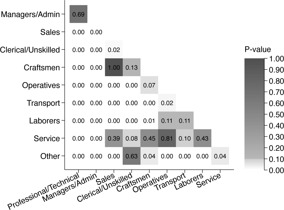
Then we run the postestimation command pheatplot to test differences between the occupation indicators (figure 3), adding the option mono to get the heat plot in grayscale color palette rather than the default color palette (see figure A1 in the supplementary online appendix).

Figure 3.

Heat plot of $p$ -values using pheatplot

. pheatplot occupation, mono

The resulting figure shows the $p$ -values of pairwise comparisons of occupation categories. If we want to export the heat plot of $p$ -values to a file, we can specify the option savegraph():

. pheatplot occupation, savegraph(p_values.pdf, replace)

(output omitted)

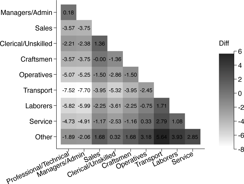
Additionally, we can specify the option differences to get a figure containing the difference between coefficients and the relative size of the differences indicated by colors (figure 4). By default, the heat plot of differences is shown without values. However we can request values by passing options along to the heat plot of differences by adding options in heatoptsb(). Here we have included values(format ()) to get differences with two decimals. Moreover, we can specify the option savetable() to store a table containing the difference in coefficients for all pairwise comparisons as well as the SEs of the differences and their $p$ -values (not shown).

• . pheatplot occupation, mono differences savetable(table_of_differences, replace)

• > heatoptsb(values(format(%9.2f)))

Figure 4.

Heat plot of differences between coefficients using pheatplot

4.3 Threshold values and color

The default behavior of the pheatplot command is to use coloring that emphasizes $p$ -values above and below some critical threshold value. By default, this threshold value is set to $p=0.10$ .However, the user can change this threshold value. In figure 5, we show an example where the threshold is set to $p=0.05$ .

Figure 5.

Heat plot of $p$ -values using pheatplot with threshold at $p=0.05$

. pheatplot occupation, mono threshold(.05)

All figures presented in this article are in grayscale using the option mono. However the default of pheatplot is to show all results in color (online appendix figure A1).

. pheatplot occupation

(output omitted)

Alternatively, the user can specify other color palettes via the heatoptsp(colors ()) option. For example, to use one of the sequential single-hue ColorBrewer palettes developed by Brewer, Hatchard, and Harrower (2003), one can use the following code (appendix figure A2):

. pheatplot occupation, heatoptsp(colors(Blues))

(output omitted)

To create a diverging color scale, one can use the following code, which also puts more emphasis on $p$ -values close to conventional threshold levels (appendix figure A3):

. pheatplot occupation, heatoptsp(colors(Orange gs15 Blue,

> ipolate(100, position(0 .10 1)) intensity(.7)))

(output omitted)

4.4 Interaction with a factor variable

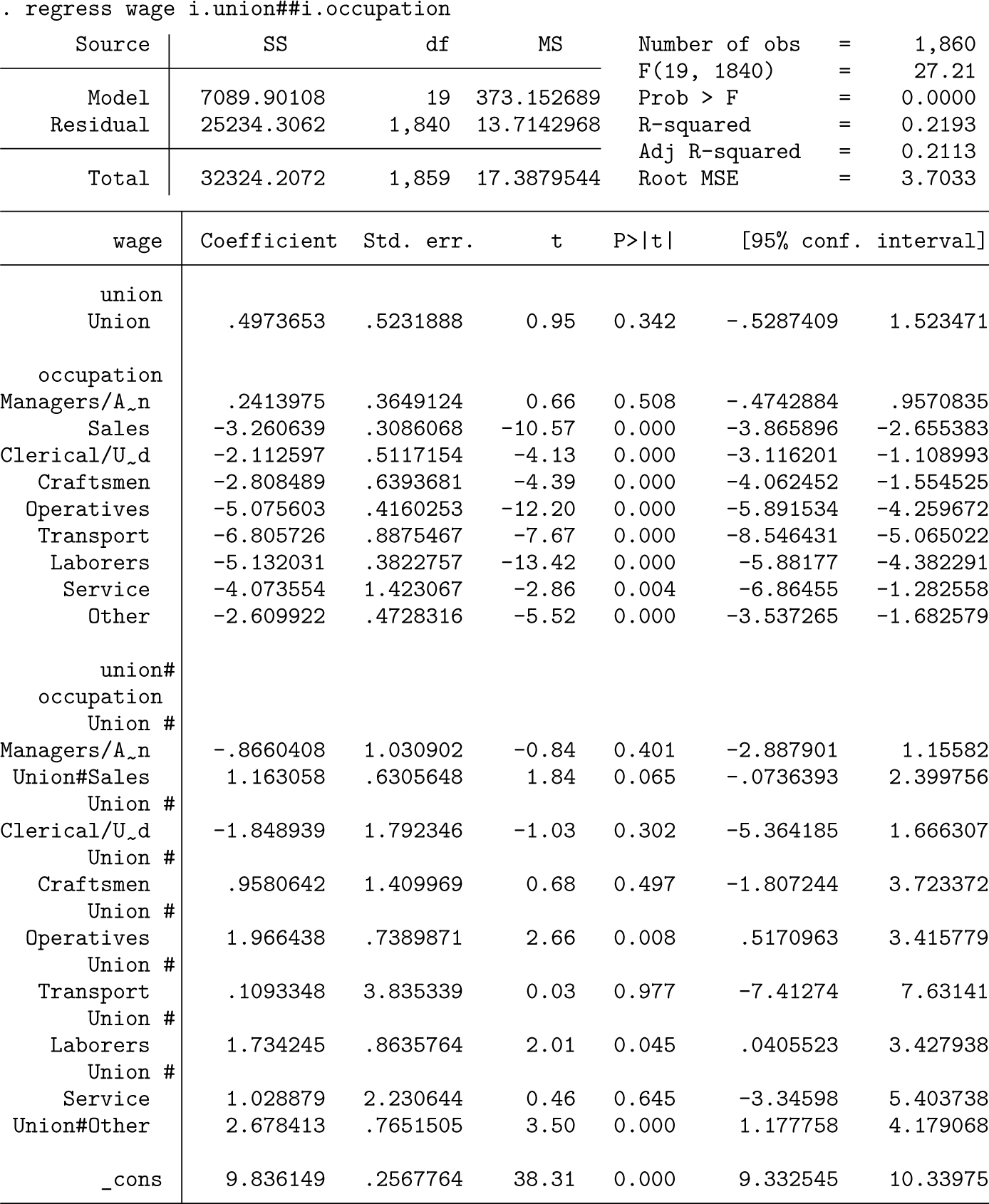
The pheatplot command can also aid the interpretation of differences in the coefficient of one variable across values of a categorical variable (that is, interaction effects). Using nlsw88.dta again, we regress wages on union and occupation, as well as the interaction between these variables, to assess the differences in union effects by occupation.

By including the option interaction(), we can test differences in the union coefficient across all occupation groups (figure 6). Note that factor-variable notation needs to be used to specify whether the interaction variable is an indicator variable (i.) or a continuous (c.) predictor.

Figure 6.

Heat plot of $p$ -values using pheatplot

. pheatplot occupation, mono interaction(i.union)

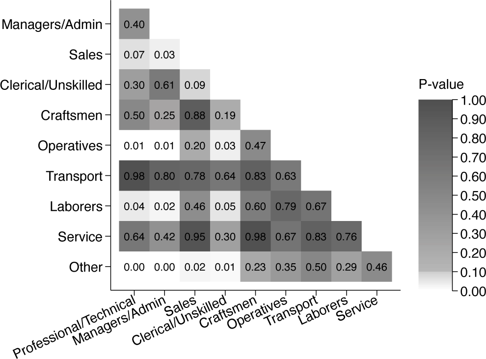
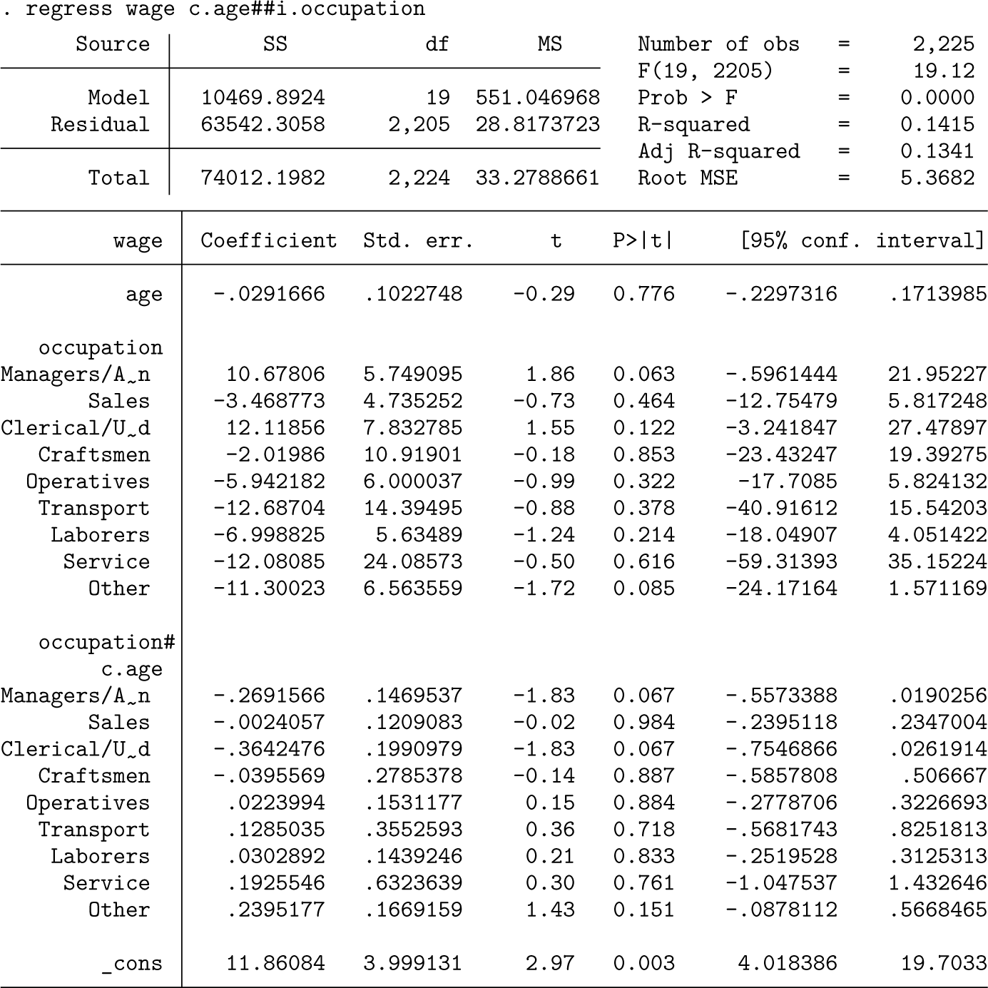
4.5 Interaction with a continuous variable

Similarly, we could be interested in differences in the coefficient of a continuous variable across categories. In the following example, we have replaced the indicator variable union with age, and we examine whether age coeficients differ by occupation (figure 7).

Figure 7.

Heat plot of $p$ -values using pheatplot

4.6 Other regression commands

While most of our examples use regress, pheatplot can also be used after other regression commands in Stata, such as logit, probit, mixed, areg, xtreg, and qreg. For example, we can use pheatplot after logistic regression (output not shown).

• logit union i.occupation

• pheatplot occupation

Moreover, pheatplot can be used after margins in some cases to plot $p$ -values and differences in average marginal effects. To plot results based on the margins command the option post must be specified in the margins command (output not shown).

logit union i.occupation##c.grade

margins, dydx(occupation) post

pheatplot occupation

The margins command in combination with pheatplot is also useful when we have interaction variables. In the following example (output not shown),we have an interaction between a categorical variable (occupation) and a binary variable (union) and want to check whether there is a difference in wages by occupation for those who are part of a union (union =1).

• regress wage i.occupation##i.union

• margins i.occupation, at(union=(1)) post

• pheatplot occupation

4.7 Customize heat plot

There are several ways to customize the heat plot of $p$ -values and the heat plot of differences. The option hexplot requests that hexagon plots are used instead of heat plots. Furthermore, pheatplot displays $p$ -values by default, but the option pvalues(off) removes the numeric display of $p$ -values (appendix figure A4).

• regress wage i.occupation

• pheatplot occupation, hexplot pvalues(off)

There are also other ways to customize the heat plots. In the following code, we have added heatoptsp (), which passes options along to the heat plot of $p$ -values. Specifically we have changed the scaling of the size of legends and cell numbers (scale ()), changed the position and look of the color ramp (ramp()), set the number of decimals of the $p$ -values to three (values ()), and changed the color palette (colors ()). The figure is shown in appendix figure A5.

pheatplot occupation, pvalues(off) heatoptsp(scale(0.7) ramp(scale(.7) ///

space(10) below label(#5) subtitle(P-value) format(%9.2f)) ///

colors(Orange gs15 Blue, ipolate(100, position(0 .10 1)) intensity(.7)) ///

values (format (%9 .3f)))

Similar changes can be made to the heat plot of differences between coefficients using the heatoptsb() option whenever the option differences is specified.

5 Conclusions

In this article, we have introduced the postestimation command pheatplot as a tool to facilitate pairwise comparisons of coefficients resulting from regression models and to assess their statistical significance, thereby helping researchers to avoid the eyeballing fallacy. Through heat plots (Jann 2019), pheatplot offers an efficient method for visually representing statistical differences between point estimates of categorical variables or differences in effects of an interaction variable by values of a categorical variable.

Furthermore, because pheatplot visualizes $p$ -values of the differences between coefficients on a continuous scale, it is tailored for comprehensively interpreting statistical significance rather than relying on arbitrary cutoffs. Thus, it serves as a useful instrument to move beyond the traditional binary $p<0.05$ significance threshold, aligning with evolving discussions in the statistical community (Bijak 2019; Nature 2019; Wasserstein, Schirm, and Lazar 2019).

However, pheatplot does not eliminate the risk of misinterpreting and abusing statistical tests. As Greenland et al.(2016) underscored in their comprehensive guide to misinterpretations, there is a widespread problem of wrongful interpretations of statistical tests, and no statistical method is exempt from this. While pheatplot does replace the binary $p$ -value thresholding with a continuous measure, it does not, on its own, prevent researchers from drawing conclusions based on arbitrary cutoffs, nor does it prevent other misinterpretations of $p$ -values (Greenland et al. 2016). Moreover, it is crucial to always interpret precise $p$ -values in conjunction with the size of the parameter estimate and the CIs rather than relying exclusively on $p$ -values.

6 Acknowledgments

We are grateful for the comments from one anonymous reviewer who helped us refine how to use color to signal statistical significance, as well as for comments and suggestions from editor Stephen Jenkins and coeditor Nick Cox. The contribution of Elisa Brini was funded by the Research Council of Norway (#300870); the contribution of Solveig Topstad Borgen was funded by the Research Council of Norway (#300917 and #314249); and the contribution of Nicolai T. Borgen was funded by the European Research Council (#818425).

7 Programs and supplemental material

To install the software files as they existed at the time of publication of this article, type

. net sj 25-1

. net install gr0099 (to install program files, if available)

. net get gr0099 (to install ancillary files, if available)

To download the pheatplot package from the Statistical Software Components Archive, type the following

. ssc install pheatplot

Supplemental Material

sj-pdf-1-stj-10.1177_1536867X251322962 - Supplemental material for Avoiding the eyeballing fallacy: Visualizing statistical differences between estimates using the pheatplot command

Supplemental material, sj-pdf-1-stj-10.1177_1536867X251322962 for Avoiding the eyeballing fallacy: Visualizing statistical differences between estimates using the pheatplot command by Elisa Brini, Solveig Topstad Borgen, and Nicolai T. Borgen in The Stata Journal

Supplemental Material

sj-txt-2-stj-10.1177_1536867X251322962 - Supplemental material for Avoiding the eyeballing fallacy: Visualizing statistical differences between estimates using the pheatplot command

Supplemental material, sj-txt-2-stj-10.1177_1536867X251322962 for Avoiding the eyeballing fallacy: Visualizing statistical differences between estimates using the pheatplot command by Elisa Brini, Solveig Topstad Borgen, and Nicolai T. Borgen in The Stata Journal