
Abstract
Item response theory models allow estimation of participant and group-mean trait scores from responses to a set of items, but estimates can be biased when participants vary in their response style. We illustrate models fit in
Introduction
Item response theory (IRT) models allow estimation of participant and group-mean trait scores from responses to a set of items (questions). The possible responses, or response set, are almost always ordered categories. IRT is much used in education for measuring student attainment (for example, https://www.oecd.org/pisa/data/pisa2018technicalreport/), where the coded response set is typically correct and incorrect. In many other settings, respondents themselves grade the response, often using a Likert scale where, for example, for the question “Do you worry about everyday things?”, the available alternatives could be never, rarely, sometimes, often, or always (Bluett-Duncan et al. 2024). Interpreting differences in questionnaire responses from different respondents usually requires that we assume that the respondents share a common understanding of both the questions and the meaning of the set of response options that they are offered. Do respondents agree on what constitutes worry rather than mere thought? Do respondents all share the same understanding of how rare is “rarely”? The assumption of a common understanding becomes increasingly difficult to make when respondents differ in their life experiences, for example, when we compare generations or populations from different cultural backgrounds or countries.
Standard IRT modeling is well covered by Stata’s own
AVs were proposed by King et al. (2004) to solve this problem in relation to the assessment of individual political efficacy. These vignettes are commonly presented via text but have also been presented orally, in pictures (Jordans et al. 2020), or through video clips (Young et al. 2020). The AV method is predicated on two measurement assumptions: vignette equivalence (all participants consider the vignettes represent the same level of trait) and response consistency (the same scale is used for self and vignette responding) (d’Uva et al. 2011). Rabe-Hesketh and Skrondal (2002) showed how
IRT models for both trait and response style
Factor model for polytomous data
Within the family of the generalized linear latent variable models (Bartholomew, Knott, and Moustaki 2011; Rabe-Hesketh, Skrondal, and Pickles 2004), factor models for poly-tomous data and IRT models provide a powerful framework for the analysis of question/naire responses. The various ways in which factor models for polytomous data can be implemented in Stata have been previously described (Raykov and Marcoulides 2018; Grant et al. 2017; Zheng and Rabe-Hesketh 2007). For the context of our empirical work in cross-cultural comparison of self-report scores, we focus here on a graded membership ordinal-response probit model.
Let yhij denote the response to the item i (i = 1,…,p), of individual j (j = 1…, N), from group h (h = l,…, H). Then the latent trait position (θhj) of individual j, from group h, is assumed to follow a conditionally normal distribution G, with a common variance


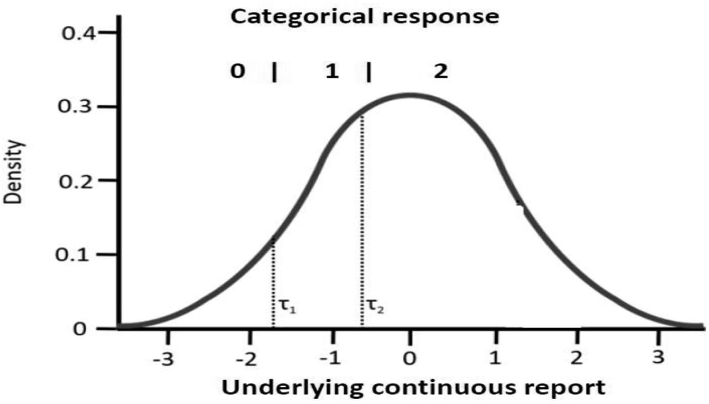
Distribution of y* with response category thresholds for a three-category response set
We now consider a setting where, in addition to a self-rating for each item, we have ratings of AVs. For each item, we may have multiple vignettes reflecting various levels of the trait under investigation. We treat variation in the ratings of the same vignette between participants as reflecting variation in response style or bias, which is modeled as another latent trait eta (
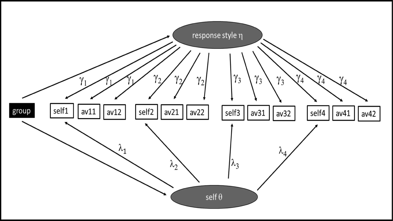
For the item responses for each participant, two latent traits now contribute to the unobserved continuous score distribution for each item, the core trait and the response style trait, extending (2) to a two-factor model


Model for
In the mean-shift (MS) model, differences in bias in group estimates are considered to arise from differences in the mean of the response style factor. The response style is assumed conditionally independent of
While the size of the response style factor and the pattern of its factor loadings across items can be of considerable interest, the motivation for much of the interest in AVs has principally been to account for systematic differences in response style that in the self-ratings may be confounded with true differences in the core trait.
On the assumption of common thresholds, (4) and (5) allow us to separate system/atic differences in the mean of the response style factor that are distinct from those systematic differences in the self-report factor.
We refer to this model as the mean-shift random (MSR) bias model M4. Restricting ση = 0 makes the response bias the same for all individuals with the same values of covariates and group, allowing the bias-adjustment terms to be included in the fixed part of the model. We call this model the MS bias model M2.
The free-thresholds model
An alternative approach to restricting rating differences to differences in the bias factor is to allow for differences in the thresholds. Rabe-Hesketh and Skrondal (2002) in their implementation of King’s CHOPIT model allow the spacing between thresholds to be a linear function of covariates via a log-link function. More easily implemented in
To summarize the models:
Model M1 is the standard probit model for ordinal self-report that allows for no reporting bias. Model M2 (MS) allows for a fixed (shared by everyone with same covariates or from same group) bias uniform across the scale or thresholds of each item. Model M3 (FT) allows bias to be different at different points along the scale of each item. Models M4 (MSR) and M5 (FTR) add individual differences in the strength of this bias (a response style factor) to models M2 and M3, respectively.
Example
Simulated data structures
A primary purpose of this article is to illustrate how different models can or cannot recover unbiased estimates of group differences in trait in the presence of response style variation of different kinds and how for some models this could be achieved with data from novel AV presentation designs that radically expand their wider use. This required us to use simulated data.
Item response generation
The simulated data consisted of p = 4 items, each with K = 3 category ordinal responses {0,1, 2} obtained by placing thresholds on Gaussian y* variates formed from the sum of contributions from independent Gaussian trait and response style and bias factors. Two groups of Nh = 500 participants were generated. Each participant provided a self-report and in most scenarios additional ratings of up to two AVs for each item. The dataset structure as it appears in Stata (long format) is
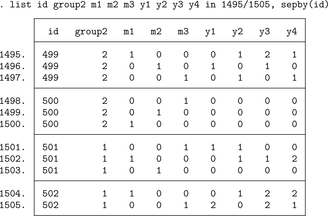
The variable id stands for the unique identifier of each of the 1,000 participants. Three dummy variables (
The factor loadings of the response-generating model, relating trait and response style to underlying response y*, varied across items but were common across groups and the same for both trait and response style, though this last was not imposed by the fitted models. The item thresholds and category boundaries varied across items.
We also simulated data where rather than the bias being introduced into the data through the y* distribution, it is introduced as differences in threshold, specifically one standard deviation group difference in the first of the two thresholds of each item. This could correspond to a difference in the interpretation of the wording used to define the first and second categories of the response set of the items, perhaps a difference in what is understood by “sometimes”. With only one of the two thresholds differing by group, there is no MS model that would match these data.
We considered four data-generating models:
G1 corresponded to analysis model M1, where there was no bias. G2 corresponded to M2, where the bias took the form of thresholds shifted uniformly. G3 corresponded to M4, where the bias was uniform across thresholds but varied between individuals. G4 corresponded to M5, where bias was present for only one of the two thresholds and the magnitude of that bias varied between individuals.
Vignette presentation design
Properly characterizing the response style of each participant requires that they respond to several vignettes for each item. This can present an excessive burden on participants. If we reduce the number of vignettes, it would seem intuitively good sense to present vignettes that were more likely to be close to the thresholds that bounded each respondents self-report and not to present those much more mild (lower-trait
Provided vignette selection is based on prior observed responses, the data missing from the unpresented vignettes conform to being missing at random and are ignorable under
Thus, in addition to scenarios with one and two vignettes for each item, we sim/ulated this approach by considering the two-vignette-per-item data with random bias but where those with self-report = 0 are presented with the first vignette and those with self-report = 2 are presented with the second vignette. Only those with intermediate self-report = 1 are presented with both vignettes. This reduced the number of vignette presentations by 39%.
The additional response burden of AVs can be entirely eliminated for the target sample if the AVs are presented instead to an entirely independent sample. To examine such a scenario, we modified our data with two vignettes so that in each group one half responded only to the self-report and one half responded only to the AVs. No one in these data responded to both self-report and AVs.
Thus, we considered five vignette availability scenarios:
D1 corresponded to self-report data only. D2 had self-report and an additional single vignette per item capable of removing response style bias. D3 had two vignettes per item and expected to improve precision and bias reduc/tion. D4 selected one or both from the available vignettes adaptively, potentially able to further improve precision and make the consistency assumption more tenable because vignettes are selected to be closer to self-report. D5 had self-report and vignettes but not from the same participants, half the sample providing self-report and half responses to AVs.
Model specification in gsem
The standard bias-naive model
The standard IRT model of (1) allows the mean of the y* distribution to vary by group, reflected in the standard factor model M1 specified in
where
The model fits two threshold parameters for each item, labeled
The MS model
The MS bias model M2 is extended for a single vignette per item by the addition of the fixed effect for dummy variable
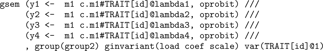
The FT model
Model M3 allows nonuniform bias along the scale (that is, at different thresholds) by the use of the multiple group option, with all parameters constrained equal across groups except for thresholds,
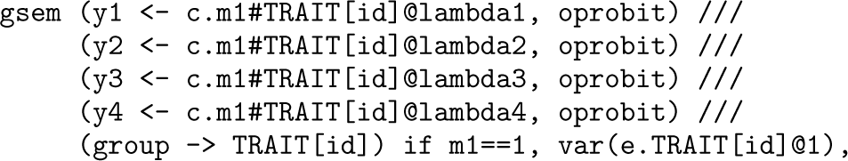
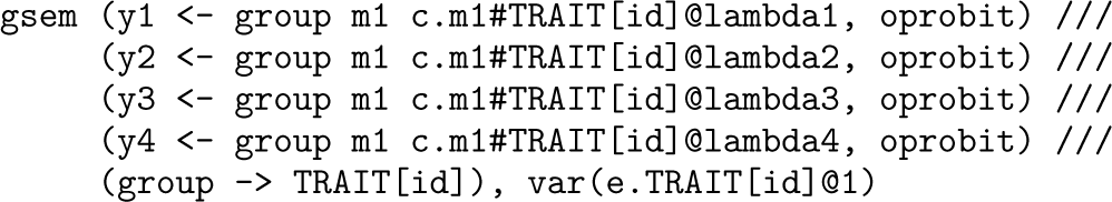
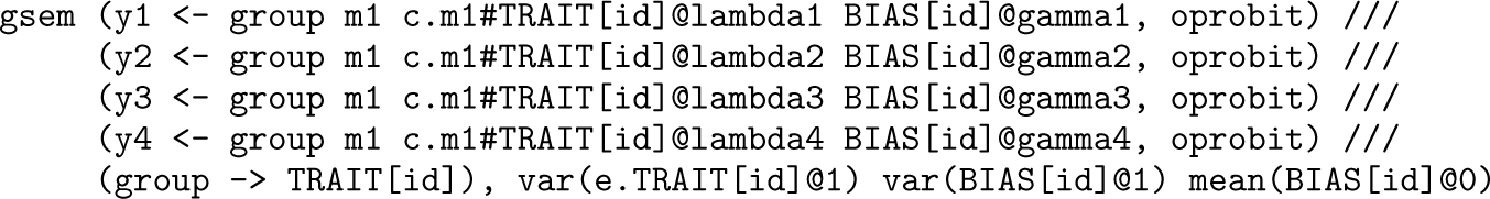
The MSR bias model
To allow for random bias variation between participants, we add a second latent variable,
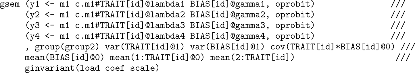
The FTR bias model
The corresponding FTR bias model M5 can be specified by
Results: Single dataset example and model comparison simulation study
Tips and tricks
The example log file illustrates the use of several options to assist in
Interpretation of parameter estimates—MSR bias model
Displayed below is the output from the first of the datasets simulated under the MSR bias model with a
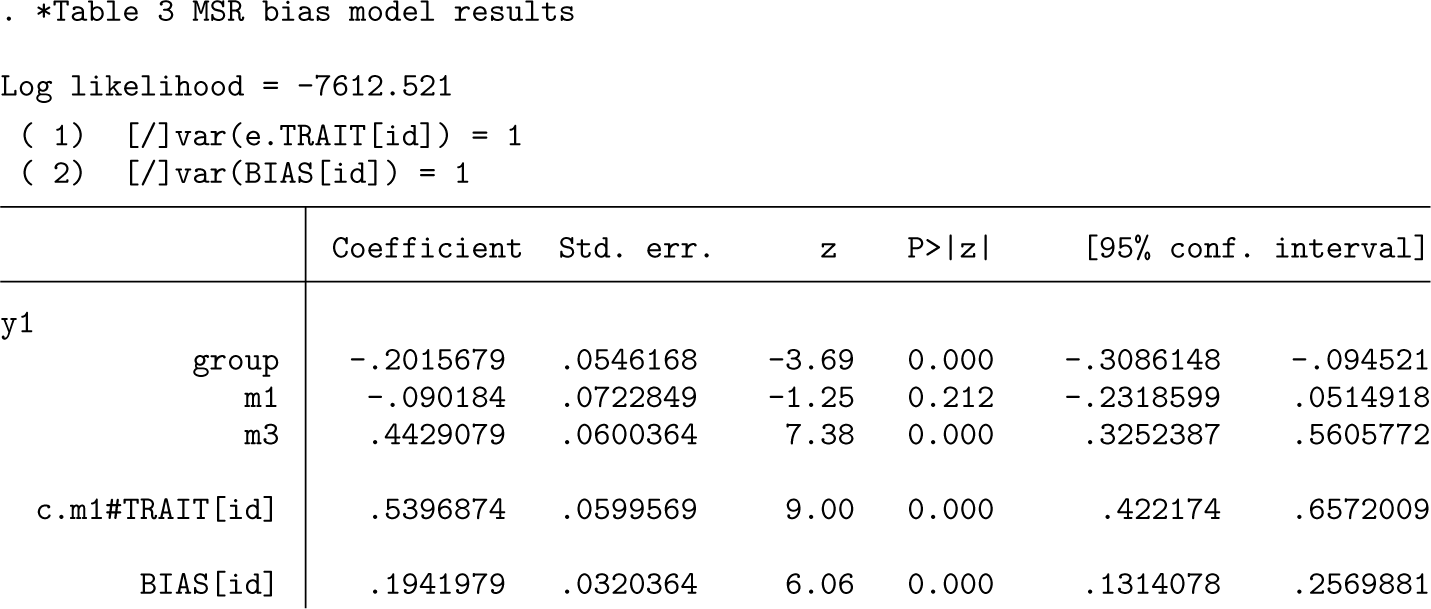
The four coefficients for
The cut coefficients near the bottom of the output are the unstandardized thresholds for the self-reporting of the four items. These were simulated to have standardized values of 0.5 and 1.5 (two thresholds for each item because the response sets have three categories with values typical of those found for symptom presence). These cutpoint coefficient estimates must be standardized by the standard deviation of
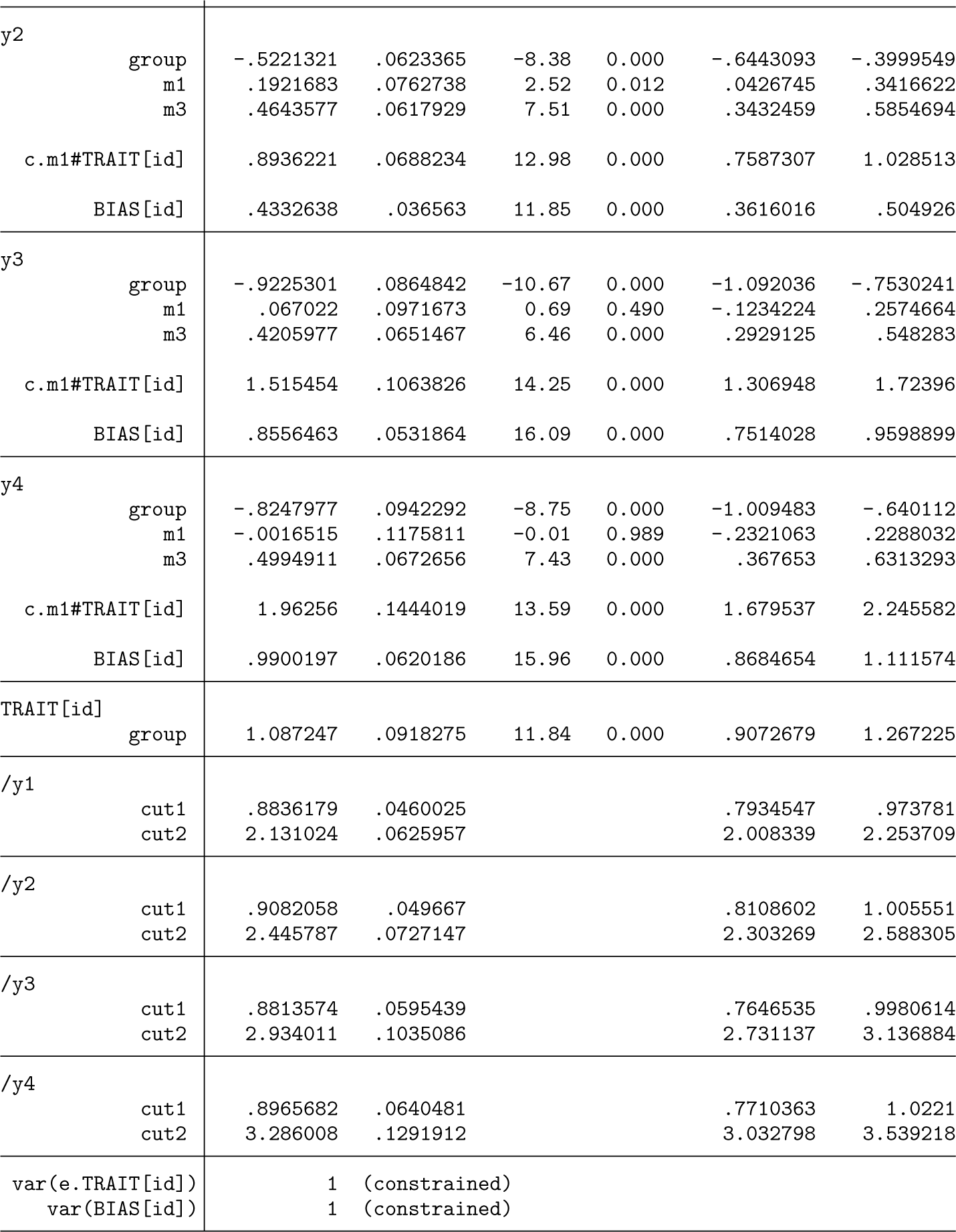
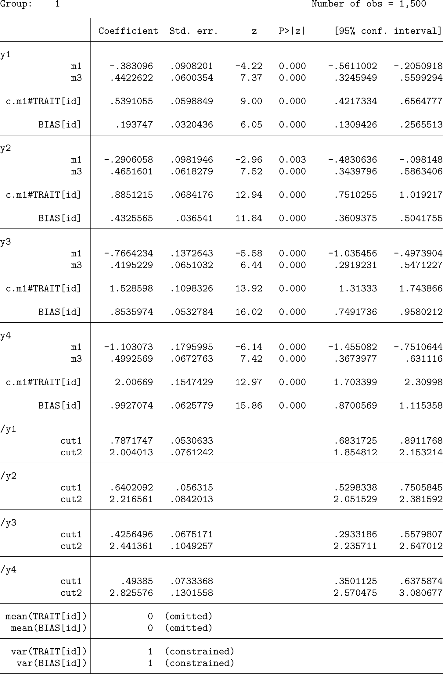
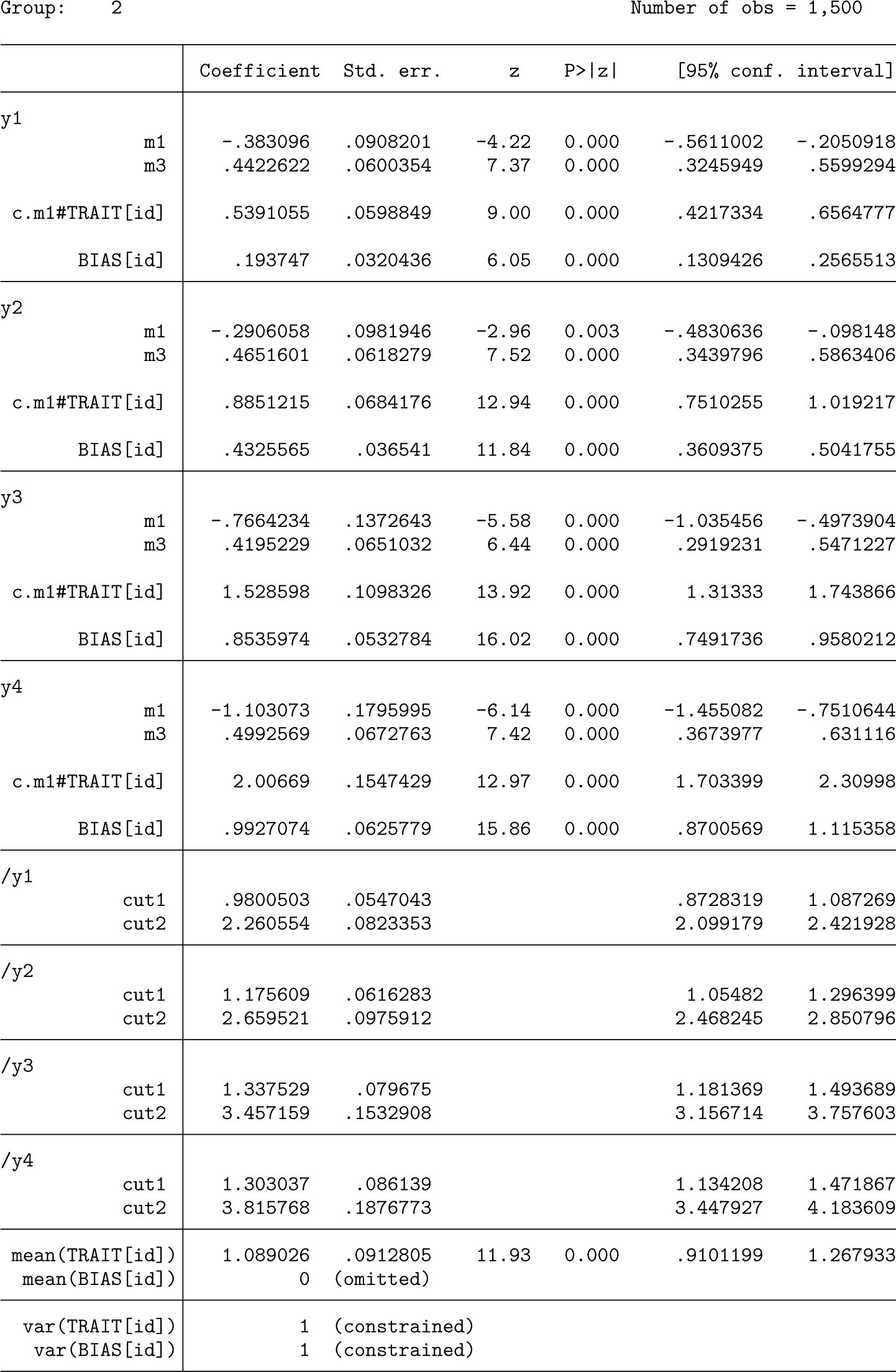
Interpretation of parameter estimates—FT model
In the FTR bias model fits shown below, there is no difference in the means of the
Model comparison simulation study
For many studies, the primary focus is on estimating covariate or group difference coefficients. In this section, we examine the performance for the estimation of a group difference in trait for five different models (M
1
to M5) when fit to data from four data-generating models (G1 to G4) and five different data availability scenarios (D1 to D5). We used Stata’s
Standard bias-naive model M1
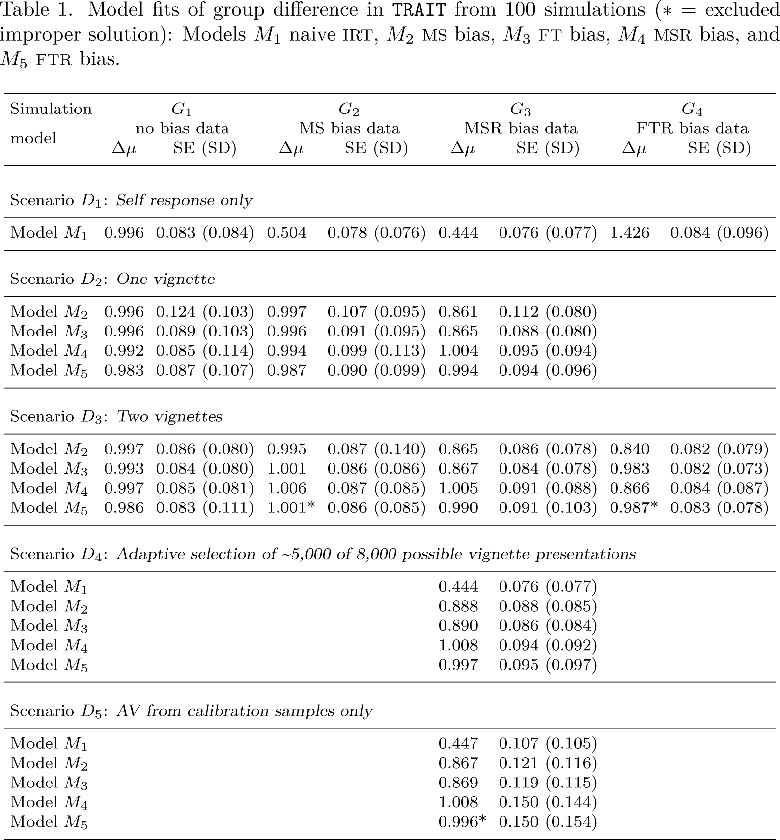
The first row of table 1 displays estimates from the standard bias-naive IRT model. Only for data-generating model G1, which has no response bias of any kind, does the average model fit of 0.996 give an unbiased estimate of the group difference (true value 1.000) in mean trait. Elsewhere, the bias is substantial, several times the standard error
Model fits of group difference in TRAIT from 100 simulations (* = excluded improper solution): Models M1 naive IRT, M2 MS bias, M3 FT bias, M4 MSR bias, and M5 FTR bias.
Model fits of group difference in
The fixed mean bias model M2 can recover an unbiased estimate of the group difference where the response style factor has zero variance (column G2), but the bias adjustment is incomplete where this is not the case (columns G3 and G4). The standard error falls from ∼0.99 to 0.86 with two vignettes rather than one vignette per item, a pattern common to all the models.
The MSR bias model M4 requires fitting both
M3 FT and M5 FTR bias models
The FT model (M3) recovers the true score with the same precision and bias as the MS (M2) model for both uniform-shift and random bias data (G2 and G3) and also for the nonuniform shift setting (G4). The FTR recovers an unbiased estimate under all data-generating models and scenarios.
Adaptive AV presentation and AV calibration sample
Evident from scenario D4 of table 1, adaptive AV selection has not changed the pattern of success in bias adjustment, with both the appropriate MS and FTR bias models providing unbiased estimates of the group difference in trait. A nearly 40% reduction in the number of AVs presented has come with only a small loss of precision, suggesting that adaptive AV selection is a more efficient study design.
We can exploit the missing-at-random assumption further and partition the participant burden by restricting the AV presentation to a subsample of participants. We can also distinguish the target samples that we wish to compare from those who complete self-report by selecting additional independent “bias calibration” samples who potentially respond only to the AVs. The self-report data from the calibration sample participants could either be ignored (as in the results we present) or included in the analysis but allowed a different mean.
For scenario D5, model convergence was poorer (85 out of the 100 simulated datasets with a further FTR estimate infeasible), but for those 85, the true group difference estimate, their standard error, and corresponding standard deviation were all satisfactorily recovered by both MS and FT models that included random bias (as the simulated data did). With half the number of self-reports (target sample n = 250 per group) and AV presentations (calibration sample n = 250 per group) of scenario D3, we would expect a doubling of the variance of the estimate. However, the reported variance for the two models increases by about 0.1502/0.0912 = 2.7, suggesting some loss of efficiency compared with having self-report and AVs from the same sample.
Conclusion
We have presented
Our work was motivated by wanting to adjust for response style in a questionnaire where the set of response alternatives offered was different for almost every item (Bluett- Duncan et al. 2024), and so all our models allowed for unconstrained response style factor loadings. Response style is often defined a priori as a particular pattern of response bias leading subjects to consistently respond in a certain way (for example, extreme, acquiescent, midpoint) (Paulhus 1991; Van Vaerenbergh and Thomas 2012), suggesting more restricted models might be appropriate, especially where the items share a common response set.
Footnotes
4
This work was supported by NICHR SI award NF-SI-0617-10120, the NICHR Maudsley Biomedical Research Centre at the South London, and Maudsley NHS Foundation Trust. The motivating study was funded jointly by the UK Medical Research Council and Indian Council for Medical Research (Grants MR/N000870/1 and ICMR/MRC-UK/2/M/2015-NCD- 1) to Helen Sharp and Andrew Pickles. Matt Bluett-Duncan was funded through a dual PhD scholarship from the University of Liverpool and the National Institute for Mental Health and Neuroscience, Bangalore.
5
About the authors
Andrew Pickles is Professor of Biostatistics and Psychological Methods at King’s College Lon/don. He has contributed to the development of the
Matt Bluett-Duncan is a postdoctoral researcher with expertise in the development of cross- cultural research methods and investigations regarding the impact of environmental exposures on fetal and child neurodevelopment.
Helen Sharp is Professor of Perinatal and Clinical Child Psychology with a research focus on the earliest origins of childhood mental health problems.
Silia Vitoratou is a senior lecturer in psychometrics and leads the Psychometrics and Measure/ment Lab at King’s College London.