On synthetic difference-in-differences and related estimation methods in Stata

Abstract

In this article, we describe a computational implementation of the synthetic difference-in-differences (SDID) estimator of Arkhangelsky et al. (2021, American Economic Review 111: 4088-4118) for Stata. SDID can be used in many circumstances where treatment effects on some particular policy or event are desired and repeated observations on treated and untreated units are available over time. We lay out the theory underlying SDID both when there is a single treatment adoption date and when adoption is staggered over time, and we discuss estimation and inference in each of these cases. We introduce the sdid command, which implements these methods in Stata, and provide several examples of use, discussing estimation, inference, and visualization of results. Along with SDID, the sdid command allows for the implementation of standard synthetic control and difference-in-differences methods in an identical framework, permitting estimation, inference, and the generation of graphical output in a computationally efficient way.

1 Introduction

There has been a recent explosion in advances in econometric methods for policy analysis. A particularly active area is estimating the impact of exposure to some particular event or policy when observations are available in a panel or repeated cross-section of groups and time (see, for example, recent surveys by de Chaisemartin and D’Hault-fauille [2022], Roth et al. [2022], and Arkhangelsky and Imbens [2023] for reviews of these methods). A modeling challenge in this setting is determining what would have happened to exposed units had they been left unexposed. Should such a counterfactual be estimable from underlying data, causal inference can be conducted by comparing outcomes in treated units with those in theoretical counterfactual untreated states under the potential-outcome framework (Holland 1986; Rubin 2005).

Many empirical studies in economics and the social sciences more generally seek to estimate effects in this setting using difference-in-differences (DID) designs. Here impacts are inferred by comparing treated units with control units, where time-invariant-level differences between units are permitted as well as general common trends. However, the drawing of causal inferences requires a parallel-trends assumption, which states that in the absence of treatment, treated units would have followed parallel paths to untreated units. Whether this assumption is reasonable in a particular context is an empirical issue. Recently, several methodologies have sought to loosen this assumption. These include procedures in which counterfactual trends can be assumed to deviate from parallel, leading to partial identification (Manski and Pepper 2018; Rambachan and Roth 2023), flexible procedures to adequately control for any prevailing differences between treated and control units (Bilinski and Hatfield 2018) often based on pretreatment periods only (Bhuller et al. 2013; Goodman-Bacon 2021), and instrumental-variables methods that explicitly consider dynamics in pretreatment periods (Freyaldenhoven, Hansen, and Shapiro 2019).

In many cases, parallel trends may be a questionable modeling assumption. One particular solution to the challenge has been the application of synthetic control (SC) methods. Early work in SC methods explores the setting of comparative case studies, where a single treated unit is observed and one wishes to construct a matched SC from a larger number of potential donor units (Abadie and Gardeazabal 2003; Abadie, Diamond, and Hainmueller 2010, 2015). These methods seek to generate a single SC from a unique convex weighting of underlying control units such that this SC is as closely matched as possible to the treated unit in pretreatment outcomes and potentially other covariates. These weights are optimally generated and fixed over time, potentially assigning zero weight to certain control units and larger weights to others. This has attracted considerable attention in both empirical applications and theoretical extensions, with recent advances including debiasing procedures (Ben-Michael, Feller, and Rothstein 2021) that can additionally house multiple treatment units (Abadie and L’Hour 2021), more flexible weighting schemes, or constant fixed differences between treated and SC units (Doudchenko and Imbens 2016; Ferman and Pinto 2021).

A recent particularly flexible modeling option that can be applied in panel-data settings seeks to bridge the DID and SC procedures. Arkhangelsky et al. (2021) propose the synthetic difference-in-differences (SDID) estimator, which combines strengths from both the DID and SC methods. Like DID models, SDID allows for treated and control units to be trending on entirely different levels prior to a reform of interest. And like SC methods, SDID seeks to optimally generate a matched control unit that considerably loosens the need for parallel-trends assumptions. Correspondingly, SDID avoids common pitfalls in standard DID and SC methods—namely, an inability to estimate causal relationships if parallel trends are not met in aggregate data in the case of DID and a requirement that the treated unit be housed within a “convex hull” of control units in the case of SC. Arkhangelsky et al. (2021) propose estimation and inference procedures, formally proving consistency and asymptotic normality of the proposed estimator. Furthermore, the authors briefly discuss several important applied points such as how their estimator can incorporate covariates and how their estimator can be applied to both multiple treatment units and even multiple treatment units that adopt treatment in different time periods.

In this article, we describe the sdid command, which implements the SDID estimator in Stata. This command allows for the simple implementation of the SDID estimator provided that a strongly balanced panel or repeated cross-section of data is available covering groups and time periods. The command, written principally in Mata, seamlessly incorporates cases where there is a single treated unit, multiple treatment units, and multiple treatment periods. It reports treatment effects laid out in Arkhangel-sky et al. (2021), additionally implementing their proposed bootstrap, jackknife, and placebo inference procedures. Several graphical output options are provided to examine the generation of the SDID estimator and the underlying optimal weight matrices. While principally written to conduct SDID estimation, the sdid command (and the SDID method) nests SC and DID as possible estimation procedures that can be easily generated to allow comparison of estimation procedures and estimates. ¹ The sdid command is written in a computationally efficient way, largely implemented in Mata and adopting effective optimization algorithms. Thus, although its main use is likely in implementing SDID methods, it is potentially a useful tool for standard SC estimation and inference.

Stata provides a rich environment for panel-based analysis in DID and SC settings, and it is useful to understand how sdid both compares with and differs from the tools currently available. For SC methods, several powerful packages exist for implementation. These include the original synth package (Abadie, Diamond, and Hainmueller 2011); synth_runner (Galiani and Quistorff 2017), which allows for the additional implementation of placebo tests permuting treatment assignment; synth2, which simplifies syntax for permutation tests including placebo tests permuting treatment time (Yan and Chen 2023); and recent extensions to SC methods such as scul (Greathouse 2022), which implements SC with a LASSO selector, and allsynth, which implements bias-correction methods (Wiltshire 2022). What sdid shares with these packages for standard SC implementation is a way to simply implement SC methods and, additionally, an ability to conduct permutation inference. What sdid does not provide out of the box is an ability to conduct placebo inference based on permutation of treatment times or recent modeling extensions implemented in allsynth and scul. For DID methods, many recent innovations exist, including Stata’s native didregress, xtdidregress, and hdidregress commands and community-contributed commands that implement a range of heterogeneity-robust DID-based estimators, including did_multiplegt (de Chaisemartin, D’Haultfauille, and Guyonvarch 2019), csdid (Rios-Avila, Sant’Anna, and Callaway 2021), did_imputation (Borusyak 2021), eventstudyinteract (Sun 2021), xtevent (Freyaldenhoven et al. 2021), stackedev (Bleiberg 2021), and jwdid (Rios-Avila 2022), as well as traditional event study designs such as eventdd (Clarke and Tapia-Schythe 2021). What sdid shares with these packages for DID estimation is an ability to estimate parameters and conduct inference accounting for time-varying rollout in the presence of heterogeneous treatment effects in a valid way. What sdid does not provide, unlike many of these routines, is a way to generate a single set of dynamic estimates and confidence intervals that are robust to time-varying events and temporally heterogeneous treatment effects. Beyond its functionality for implementing both SC and DID, the principal contribution of sdid is that it allows for estimation, inference, and visualization for SDID that are not available elsewhere.

In introducing the sdid command in this article, we first provide a primer on the core methodological points of SDID (as well as comparisons with DID and SC) and then describe how these procedures extend to a setting where treatment adoption occurs over multiple time periods. We then lay out the command syntax of sdid and the elements that are returned to the user. We provide several examples to illustrate the use of the SDID method in Stata. One is based on a well-known example of California’s passage of Proposition 99, an antismoking measure previously presented in Abadie, Diamond, and Hainmueller (2010) and Arkhangelsky et al. (2021) in which a single state adopts a treatment at a given time. Another example is where exposure to a policy occurs at multiple periods: the case of parliamentary gender quotas studied by Bhalotra et al. (2023). We conclude by making several practical points on the computational implementation of this estimator and briefly discussing potential future areas of work.

2 Methods

2.1 The canonical SDID procedure

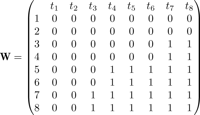
The SDID procedure was developed in Arkhangelsky et al. (2021), and we lay out its principal details here. As input, SDID requires a balanced panel of N units or groups, observed over T time periods. An outcome, denoted Y_it, is observed for each unit i in each period t. Some (but not all) of these observations are treated with a specific binary variable of interest, denoted W_it. W_it = 1 if observation i is treated by time t; otherwise, W_it = 0 if observation i is untreated at time t. Here we assume that there is a single adoption period for treated units, which Arkhangelsky et al. (2021) refer to as a “block treatment assignment”. In section 2.3, we extend this to a “staggered adoption design” (Athey and Imbens 2022), where treated units adopt treatment at varying points. A key element of both of these designs is that once treated, units are assumed to remain exposed to treatment thereafter. In the particular setting of SDID, no always-treated units can be included in estimation. For estimation to proceed, we require at least two pretreatment periods off of which to determine control units. In practice, for generating good matched controls, more pretreatment periods are required (refer to the discussion in section 5).

The goal of SDID is to consistently estimate the causal effect of receipt of policy or treatment W_it (an average treatment effect on the treated, or ATT), even if we do not believe in the parallel-trends assumption between all treatment and control units on average. Estimation of the ATT proceeds as follows:

$$({\hat{\tau }}^{\mathrm{SDID}},\hat{\mu },\hat{\alpha },\hat{\beta })=\underset{\tau ,\mu ,\alpha ,\beta }{\arg min}\left\{\sum _{i=1}^N\sum _{t=1}^T{(Y_{it}-\mu -{\alpha }_i-{\beta }_t-W_{it}\tau )}^2{\hat{\omega }}_i^{\mathrm{SDID}}{\hat{\lambda }}_t^{\mathrm{SDID}}\right\}(1)$$

(1)

The estimand is the ATT, generated from a two-way fixed-effects regression, with optimally chosen weights ${\hat{\omega }}_i^{\mathrm{SDID}}$ and ${\hat{\lambda }}_t^{\mathrm{SDID}}$ , which are discussed below. Note that here this procedure flexibly allows for shared temporal aggregate factors given the estimation of time-fixed effects β_t and time-invariant unit-specific factors given the estimation of unit fixed effects a_i. As is standard in fully saturated fixed-effects models, one a_i and one β_t fixed effect are normalized to zero to avoid multicollinearity. The presence of unit-fixed effects implies that SDID will simply seek to match treated and control units on pretreatment trends and not necessarily on both pretreatment trends and levels, allowing for a constant difference between treatment and control units.

In this setting, it is illustrative to consider how the SDID procedure compares with the traditional SC method of Abadie, Diamond, and Hainmueller (2010), as well as the baseline DID procedure. The standard DID procedure consists of precisely the same twoway fixed-effects ordinary least-squares (OLS) procedure, simply assigning equal weights to all time periods and groups:

$$({\hat{\tau }}^{\mathrm{DID}},\hat{\mu },\hat{\alpha },\hat{\beta })=\underset{\tau ,\mu ,\alpha ,\beta }{\arg min}\left\{\sum _{i=1}^N\sum _{t=1}^T{(Y_{it}-\mu -{\alpha }_i-{\beta }_t-W_{it}\tau )}^2\right\}(2)$$

(2)

The SC, on the other hand, maintains optimally chosen unit-specific weights ω (as laid out below). However, it does not seek to optimally consider time periods via time weights and omits unit-fixed effects α_i, implying that the SC and treated units should maintain approximately equivalent pretreatment levels and trends.

$$({\hat{\tau }}^{\mathrm{SC}},\hat{\mu },\hat{\beta })=\underset{\tau ,\mu ,\beta }{\arg min}\left\{\sum _{i=1}^N\sum _{t=1}^T{(Y_{it}-\mu -{\beta }_t-W_{it}\tau )}^2{\hat{\omega }}_i^{\mathrm{SC}}\right\}(3)$$

(3)

From (2)–(3), it is clear that the SDID procedure offers greater flexibility than both the DID and SC procedures; in the case of DID, it permits a violation of parallel trends in aggregate data, and in the case of SC, it both additionally seeks to optimally weight time periods when considering counterfactual outcomes and allows for level differences between treatment and control groups.

The selection of unit weights, ω, as inputs to (1) [and (3)] seeks to ensure that comparison is made between treated units and controls that were approximately following parallel trends prior to the adoption of treatments. The selection of time weights, λ, in the case of SDID seeks to draw more weight from pretreatment periods that are more similar to posttreatment periods in the sense of finding a constant difference between each control unit’s posttreatment average and pretreatment weighted averages across all selected controls. Specifically, as laid out in Arkhangelsky et al. (2021), unit-specific weights are found by resolving

$$(\widehat{{\omega }_0},{\hat{\omega }}^{\mathrm{SDID}})=\underset{{\omega }_0\in \mathbb{R},\omega \in \mathrm{\Omega }}{\arg min}\sum _{t=1}^{T_{\mathrm{pre}}}{\left({\omega }_0+\sum _{i=1}^{N_{\mathrm{co}}}{\omega }_i{Y}_{it}-{\displaystyle \frac{1}{N_{\mathrm{tr}}}\sum _{i=N_{\mathrm{co}}+1}^N{Y}_{it}}\right)}^2+{\varsigma }^2{T}_{\mathrm{Pre}}\Vert \omega {\Vert }_2^2(4)$$

(4)

where

$$\mathrm{\Omega }=\left\{\omega \in {\mathbb{R}}_{+}^N,\mathrm{with}\sum _{i=1}^{N_{\mathrm{co}}}{\omega }_i=1\mathrm{and}{\omega }_i={\displaystyle \frac{1}{N_{\mathrm{tr}}}\mathrm{for}\mathrm{all}i=N_{\mathrm{co}}+1,\dots ,N}\right\}$$

$\Vert \omega {\Vert }_2$ refers to the Euclidean norm, and ζ is a regularization parameter laid out in Arkhangelsky et al. (2021, 4091–4092). For the sake of completion, this regularization parameter is calculated as $\varsigma =(N_{\mathrm{tr}}\times T_{\mathrm{post}}{)}^{1/4}\hat{\sigma }$ , where

$${\hat{\sigma }}^2={\displaystyle \frac{1}{N_{\mathrm{co}}(T_{\mathrm{pre}}-1)}\sum _{i=1}^{N_{\mathrm{co}}}\sum _{t=1}^{T_{\mathrm{pre}}-1}{({\mathrm{\Delta }}_{it}-\overline{\mathrm{\Delta }})}^2(5)}$$

(5)

$$\begin{array}{rl}& {\mathrm{\Delta }}_{it}=Y_{i,(t+1)}-Y_{it}\\ & \overline{\mathrm{\Delta }}={\displaystyle \frac{1}{N_{\mathrm{co}}(T_{\mathrm{Pre}}-1)}\sum _{i=1}^{N_{\mathrm{co}}}\sum _{t=1}^{T_{\mathrm{Pre}}-1}{\mathrm{\Delta }}_{it}}\end{array}$$

This regularization parameter is shown to be theoretically motivated and have good performance in Arkhangelsky et al. (2021) and thus is adopted by default in sdid, but options allow for this parameter to be varied.

This procedure leads to a vector of N_co nonnegative weights plus an intercept ω₀. The weights ω_i for all $i\in \{1,\dots ,N_{\mathrm{co}}\}$ imply that absolute difference between control and treatment trend units should be minimized over all pretreatment periods, while ω₀ initially allows for a constant difference between treatment and controls over time. Together, these imply that units will follow parallel pretrends, though provided ω₀ ≠ 0, not identical pretrends.

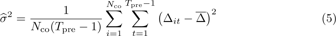
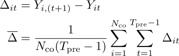
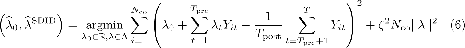
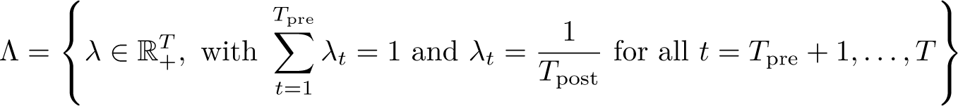
For time weights, a similar procedure is followed, finding weights that minimize the objective function

$$(\widehat{{\lambda }_0},{\hat{\lambda }}^{\mathrm{SDID}})=\underset{{\lambda }_0\in \mathbb{R},\lambda \in \mathrm{\Lambda }}{\arg min}\sum _{i=1}^{N_{\mathrm{co}}}{\left({\lambda }_0+\sum _{i=1}^{T_{\mathrm{pre}}}{\lambda }_t{Y}_{it}-{\displaystyle \frac{1}{T_{\mathrm{post}}}\sum _{t=T_{\mathrm{pre}}+1}^T{Y}_{it}}\right)}^2+{\varsigma }^2{N}_{\mathrm{co}}{\Vert \lambda \Vert }^2$$

(6)

where

$$\mathrm{\Lambda }=\left\{\lambda \in {\mathbb{R}}_{+}^T,\mathrm{with}\sum _{t=1}^{T_{\mathrm{pre}}}{\lambda }_t=1\mathrm{and}{\lambda }_t={\displaystyle \frac{1}{T_{\mathrm{post}}}\mathrm{for}\mathrm{all}t=T_{\mathrm{pre}}+1,\dots ,T}\right\}$$

where the final term in (6) is a very small regularization term to ensure uniqueness of time weights, where $\zeta =1\times {10}^{-6}\hat{\sigma }$ and $\hat{\sigma }$ is defined as in (5). Again, this parameter is adopted by default in computational implementations but can be adjusted.

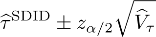
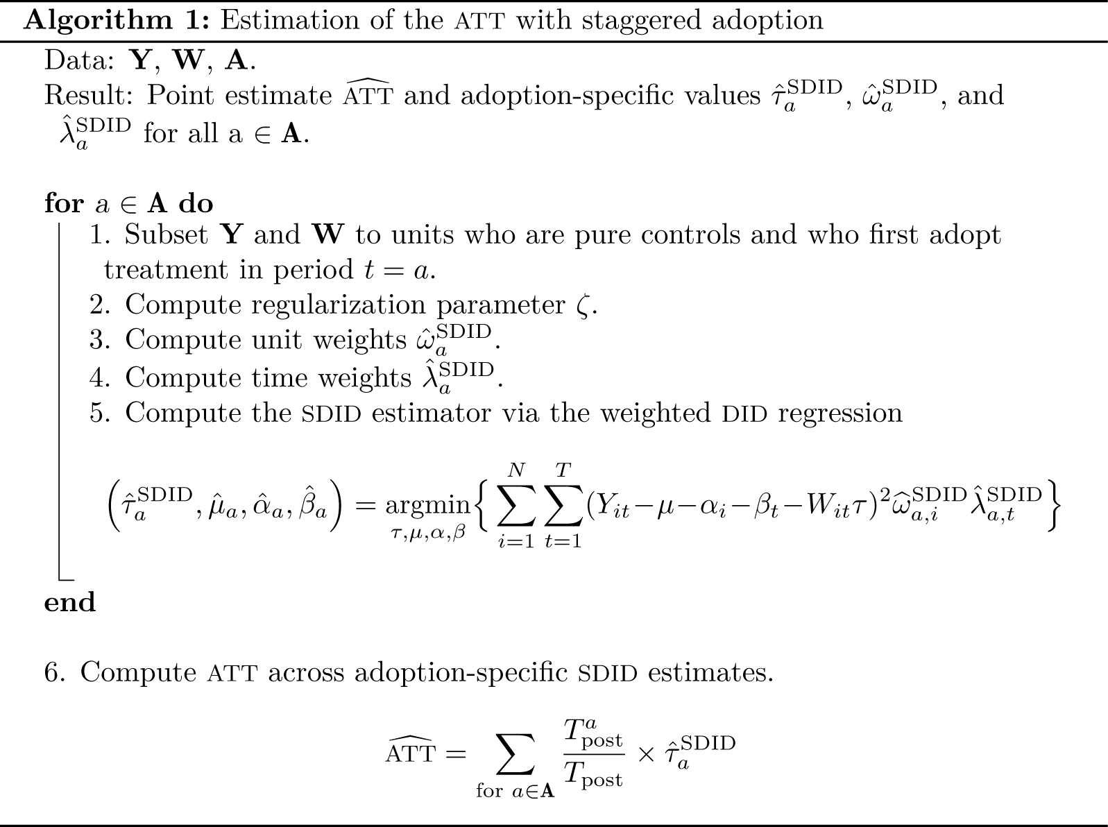
This estimation procedure is summarized in Arkhangelsky et al. (2021, algo. 1), reproduced in online appendix A1 for ease of access. Arkhangelsky et al. (2021) also prove that the estimator is asymptotically normal, suggesting that confidence intervals on τ can be constructed as

$${\hat{\tau }}^{\mathrm{SDID}}\pm z_{\alpha /2}\sqrt{\widehat{V_{\tau }}}$$

where zα/2 refers to the inverse normal density function at percentile α/2 should one wish to compute 1 − α confidence intervals. These confidence intervals thus simply require an estimate of the variance of τ, ${\hat{V}}_{\tau }$ . Arkhangelsky et al. (2021) propose three specific procedures to estimate this variance: a block bootstrap, a jackknife, or a permutation-based approach.

The block (also known as clustered) bootstrap approach consists of taking some large number, B, of bootstrap resamples over units, where units i are the resampled blocks in the block bootstrap procedure. Provided that a given resample does not consist entirely of treated or control units, the quantity ${\hat{\tau }}^{\mathrm{SDID}}$ is reestimated and denoted as ${\hat{\tau }}_{(b)}^{\mathrm{SDID}}$ for each bootstrap resample. The bootstrap variance ${\hat{V}}_{\tau }^{(b)}$ is then calculated as the variance of resampled estimates ${\hat{\tau }}_{(b)}^{\mathrm{SDID}}$ across all B resamples. The bootstrap algorithm is defined in Arkhangelsky et al. (2021, algo. 2), reproduced in online appendix A1. This bootstrap procedure is observed in simulation to have particularly good properties but has two particular drawbacks, justifying alternative inference procedures. The first is that it may be computationally costly, given that in each bootstrap resample, the entire SDID procedure is reestimated, including the estimation of optimal weights. This is especially computationally expensive when working with large samples or when covariates are included, as discussed more at length below. The second is that formal proofs of asymptotic normality rely on the number of treated units being large, and thus, estimated variance and confidence intervals may be unreliable when there are few treated units.

An alternative method that significantly reduces the computational burden inherent in the bootstrap is estimating a jackknife variance for ${\hat{\tau }}^{\mathrm{SDID}}$ . This procedure consists of iterating over all units in the data, removing the given unit in each iteration, and recalculating ${\hat{\tau }}^{\mathrm{SDID}}$ , denoted ${\hat{\tau }}_{(-i)}^{\mathrm{SDID}}$ , maintaining fixed the optimal weights for ω and λ calculated in the original SDID estimate. The jackknife variance, ${\hat{V}}_{\tau }^{(\mathrm{jack})}$ , is then calculated based on the variance of all ${\hat{\tau }}_{(-i)}^{\mathrm{SDID}}$ estimates, following Arkhangelsky et al. (2021, algo. 3) (refer to the online appendix A1). In this case, each iteration saves on recalculating optimal weights and, as documented by Arkhangelsky et al. (2021), provides a variance leading to conservative confidence intervals without the computational burden imposed by the bootstrap. Once again, asymptotic normality relies on there being many treated units, and in particular, if only 1 treated unit is observed—as is often the case in comparative case studies—the jackknife will not even be defined given that a ${\hat{\tau }}_{(-i)}^{\mathrm{SDID}}$ term will be undefined when removing the single treated unit.

Given limits to these inference options when there are few treated units, an alternative placebo (or permutation-based) inference procedure is proposed. This consists of first conserving just the control units and then randomly assigning the same treatment structure to these control units as a placebo treatment. Based on this placebo treatment, we then reestimate ${\hat{\tau }}^{\mathrm{SDID}}$ , denoted ${\hat{\tau }}_{(p)}^{\mathrm{SDID}}$ . This procedure is repeated many times, giving rise to a vector of estimates, ${\hat{\tau }}_{(p)}^{\mathrm{SDID}}$ ; the placebo variance, ${\hat{V}}_{\tau }^{(\mathrm{placebo})}$ , can be estimated as the variance of this vector. This is formally defined in Arkhangelsky et al. (2021, algo. 4) and the online appendix A1. Note that in the case of this placebo-based variance, homoskedasticity across units is required, given that the variance is based off placebo assignments of treatment made only within the control group.

2.2 Conditioning on covariates

So far, we have limited exposition to cases where one wishes to study outcomes Y_it and their evolution in treated and SC units. However, in certain settings, it may be of relevance to condition on exogenous time-varying covariates X_it. Arkhangelsky et al. (2021) note that in this case, we can proceed by applying the SDID algorithm to the residuals calculated as

$$Y_{it}^{res}=Y_{it}-X_{it}\hat{\beta }(7)$$

(7)

where $\hat{\beta }$ comes from regression of Y_it on X_it. This procedure, in which the SDID process will be applied to the residuals $Y_{it}^{\mathrm{res}}$ , is different from the logic of SCs following Abadie, Diamond, and Hainmueller (2010). In Abadie, Diamond, and Hainmueller’s (2010) conception, when covariates are included, the SC is chosen to ensure that these covariates are as closely matched as possible between treated and SC units. However, in the SDID conception, covariate adjustment is viewed as a preprocessing task that removes the impact of changes in covariates from the outcome Y_it prior to calculating the SC. Along with their article, Arkhangelsky et al. (2021) provide an implementation of their algorithm in R (Arkhangelsky et al. 2019), and in practice, they condition out these variables X_it by finding $\hat{\beta }$ within an optimization procedure that additionally allows for the efficient calculation of optimal weights ω and λ. In the sdid code described below, we follow Arkhangelsky et al. (2019) in implementing this efficient optimization procedure (the Frank and Wolfe [1956] solver). However, there are several potential complications that can arise in this manner of dealing with covariates, and thus, alternative procedures are also available.

A first potential issue is purely numerical. In the Frank-Wolfe solver discussed above, a minimum point is assumed to be found when successive iterations of the solver lead to arbitrarily small changes in all parameters estimated. ² Where these parameters include coefficients on covariates, the solution found for (1) can be sensitive to the scaling of covariates in extreme cases. Particularly, this occurs when covariates have very large magnitudes and variances. In such cases, the inclusion of covariates in (1) can cause optimization routines to suggest solutions that are not actually globally optimal, given that successive movements in $\hat{\beta }$ can be very small. In extreme cases, this can imply that when multiplying all variables X_it by a large constant value, the estimated treatment effect can vary. While this issue can be addressed by using smaller tolerances for defining stopping rules in the optimization procedure, it can be addressed more simply if all covariates are first restandardized as z scores, implying that no very-high-variance variables are included, while capturing the same underlying variation in covariates.

A second (and potentially more complicated) point is described by Kranz (2022). He notes that in certain settings, specifically where the relationship between covariates and the outcome vary over time differentially in treatment and control groups, the procedure described above may fail to capture the true relationship between covariates and the outcome of interest and may subsequently lead to bias in estimated treatment effects. He proposes a slightly altered methodology of controlling for covariates. Namely, his suggestion is to first estimate a two-way fixed-effects regression of the dependent variable on covariates (plus time- and unit-fixed effects) using only observations that have yet to be exposed to treatment, that is, subsetting to observations for which W_it = 0. Based on the regression $Y_{it}=X_{it}\beta +{\mu }_i+{\lambda }_t+{\epsilon }_{it}$ for units with W_it = 0,coefficients $\hat{\beta }$ estimated by OLS can be used to follow the procedure in (7), and SDID can then be conducted. An additional benefit of this method is that unlike the optimized method described previously, $\hat{\beta }$ is calculated in a single step via OLS rather than in an iterative optimization procedure, which often leads to substantial speedups in computation time.

We document these methods based on several empirical examples in the following section. Note that regardless of which procedure one uses, the implementation of SDID follows the suggestion laid out in Arkhangelsky et al. (2021, n. 4) and (7) above. What varies between the former and the latter procedures discussed here is the manner with which one estimates coefficients on covariates, $\hat{\beta }$ , in a preprocessing step.

2.3 The staggered adoption design

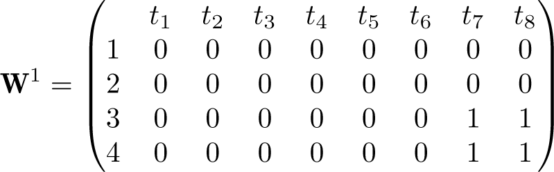
The design discussed up to this point assumes block assignment or that all units are either controls or treated in a single unit of time. However, Arkhangelsky et al. (2021, app. A) note that this procedure can be extended to a staggered adoption design, where treated units adopt treatment at varying moments of time. Here we lay out the formal details related to the staggered adoption design, focusing first on estimation of an aggregate treatment effect and then on extending the three inference procedures laid out previously into a staggered adoption setting. This proposal is one potential way to deal with staggered adoption settings, though there are other possible manners to proceed—see, for example, Ben-Michael, Feller, and Rothstein (2021) or Arkhangelsky et al. (2021, app. A). When there are few pure control units, this proposal may not necessarily be very effective given challenges in finding appropriate counterfactuals for each adoption-specific period.

Estimation. Unlike the block assignment case where a single pretreatment-versus-post-treatment date can be used to conduct estimation, in the staggered adoption design, multiple adoption dates are observed. Consider, for example, the treatment matrix below. It consists of eight units, two of which (1 and 2) are untreated and six of which are treated but at varying points.

$$\mathbf{W}\mathbf{=}\left(\begin{array}{ccccccccc}& t_1& t_2& t_3& t_4& t_5& t_6& t_7& t_8\\ 1& 0& 0& 0& 0& 0& 0& 0& 0\\ 2& 0& 0& 0& 0& 0& 0& 0& 0\\ 3& 0& 0& 0& 0& 0& 0& 1& 1\\ 4& 0& 0& 0& 0& 0& 0& 1& 1\\ 5& 0& 0& 0& 1& 1& 1& 1& 1\\ 6& 0& 0& 0& 1& 1& 1& 1& 1\\ 7& 0& 0& 1& 1& 1& 1& 1& 1\\ 8& 0& 0& 1& 1& 1& 1& 1& 1\end{array}\right)$$

This staggered treatment matrix, W, can be broken down into adoption-date-specific matrices (W¹, W², and W³) or generically (W¹,…,W ^A , where A indicates the number of distinct adoption dates). Additionally, a row vector A consisting of A elements contains these distinct adoption periods. In this specific setting, where units first adopt treatment in periods t₃ (units 7 and 8), t₄ (units 5 and 6), and t₇ (units 3 and 4), the adoption date vector consists simply of periods 3, 4, and 7.

$$\mathbf{A}=(\begin{array}{ccc}3& 4& 7\end{array})$$

Finally, adoption-specific matrices W¹–W³ consist simply of pure treated units and units that adopt in this specific period, as shown below:

$${\mathbf{W}}^1=\left(\begin{array}{ccccccccc}& t_1& t_2& t_3& t_4& t_5& t_6& t_7& t_8\\ 1& 0& 0& 0& 0& 0& 0& 0& 0\\ 2& 0& 0& 0& 0& 0& 0& 0& 0\\ 3& 0& 0& 0& 0& 0& 0& 1& 1\\ 4& 0& 0& 0& 0& 0& 0& 1& 1\end{array}\right)$$

$${\mathbf{W}}^2=\left(\begin{array}{ccccccccc}& t_1& t_2& t_3& t_4& t_5& t_6& t_7& t_8\\ 1& 0& 0& 0& 0& 0& 0& 0& 0\\ 2& 0& 0& 0& 0& 0& 0& 0& 0\\ 5& 0& 0& 0& 1& 1& 1& 1& 1\\ 6& 0& 0& 0& 1& 1& 1& 1& 1\end{array}\right)$$

$${\mathbf{W}}^3=\left(\begin{array}{ccccccccc}& t_1& t_2& t_3& t_4& t_5& t_6& t_7& t_8\\ 1& 0& 0& 0& 0& 0& 0& 0& 0\\ 2& 0& 0& 0& 0& 0& 0& 0& 0\\ 7& 0& 0& 1& 1& 1& 1& 1& 1\\ 8& 0& 0& 1& 1& 1& 1& 1& 1\end{array}\right)$$

As laid out in Arkhangelsky et al. (2021, app. A), the ATT can then be calculated by applying the SDID estimator to each of these three adoption-specific samples and calculating a weighted average of the three estimators, where weights are assigned based on the relative number of treated units and time periods in each adoption group. Generically, this ATT is calculated based on adoption-specific SDID estimates as

$$\widehat{\mathrm{ATT}}=\sum _{\mathrm{for}a\in \mathbf{A}}{\displaystyle \frac{T_{\mathrm{post}}^a}{T_{\mathrm{post}}}\times {\hat{\tau }}_a^{\mathrm{SDID}}}(8)$$

(8)

where T_post refers to the total number of posttreatment periods observed in treated units. This estimation procedure is laid out formally in algorithm 1 below.

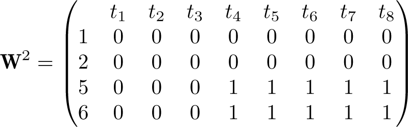
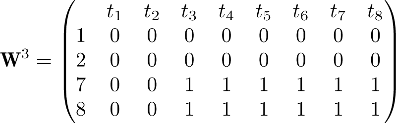
Note that in this case, while the parameter interest is likely the treatment-effect ATT or adoption-specific ${\tau }_a^{\mathrm{SDID}}$ parameters, each adoption period is associated with an optimal unit and time weight vector ${\omega }_a^{\mathrm{SDID}}$ and ${\lambda }_a^{\mathrm{SDID}}$ , which can be returned following estimation.

Inference. In the staggered adoption design, estimated treatment effects are simply multiperiod extensions of the underlying SDID algorithm, in each case working with the relevant pure control and treated subsample. Thus, inference can be conducted in the staggered adoption design under similar resample or placebo procedures. Here we discuss inference following each of the bootstrap, jackknife, or placebo procedures laid out in Arkhangelsky et al. (2021), applied to a staggered adoption setting. We note that in this design, it is likely the case that one wishes to conduct inference on the treatment effect ATT from (8). Thus, below we propose inference details for this estimand, additionally noting that standard errors and confidence intervals on adoption-specific SDID parameters ${\tau }_a^{SDID}$ come built in as part of these procedures.

Consider first the case of bootstrap inference. Suppose that one wishes to estimate standard errors or generate confidence intervals on the global treatment-effect ATT. A bootstrap procedure can be conducted based on many clustered bootstrap resamples over the entire initial dataset, where in each case, a resampled ATT estimate ${\widehat{\mathrm{ATT}}}^b$ is generated following algorithm 1. Based on many such resampled estimates, the bootstrap variance can be calculated as the variance of these resamples. We lay out the bootstrap variance estimate below in algorithm 2.

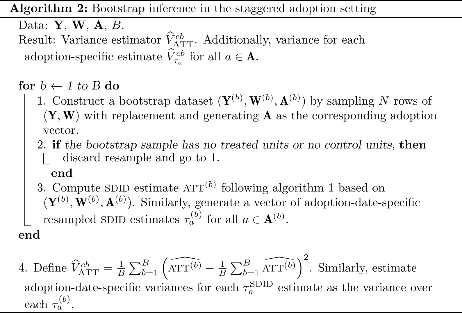
Note that as in the block treatment design, this bootstrap procedure requires the number of treated units to grow with N within each adoption period. Thus, if very few treated units exist for certain adoption periods, placebo inference is likely preferable. Similarly, as laid out in the block treatment design, the bootstrap procedure reestimates optimal weight matrices in each resample and can be computationally expensive in cases where samples are large.

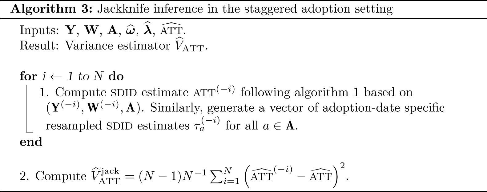
An alternative inference procedure is the jackknife, which is less computationally intensive but similarly based on asymptotic arguments with many states and treated units. Here optimal weight matrices calculated for each adoption-specific estimate ${\tau }_a^{SDID}$ in algorithm 1 are treated as fixed and provided as inputs to a jackknife procedure described below in algorithm 3. Below, these matrices, which consist of weights for each adoption period $\mathrm{a}\in \mathrm{A}$ are denoted as ω, λ. ³ Note that in algorithm 3, notation (—i) refers to a standard jackknife estimator, removing a single state (i) in each iteration. When i refers to a treated unit, the ATT will be calculated removing this particular treated unit. Therefore, the jackknife estimator will not be defined when any single adoption period has only one treated unit because in this case, ${\widehat{{\tau }_a}}^{(-\mathrm{i})}$ will not be defined.

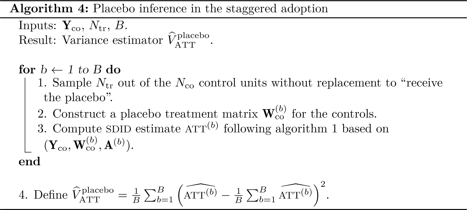
Finally, when there are few treated units and concerns related to the validity of the previous variance estimators exist, the placebo inference procedure defined in algorithm 4 can be used. Here this is defined for the staggered adoption case, generalizing algorithm 4 of Arkhangelsky et al. (2021). To conduct this procedure, placebo treatments are randomly assigned based on the actual treatment structure but only to the control units. Based on these placebo assignments, placebo values for ATT are generated that can be used to calculate the variance as laid out in algorithm 4. Note that such a procedure will be feasible only when there are strictly more control units than treated units (or, hence, placebo assignments will not be feasible) and, as laid out in Arkhangelsky et al. (2021) and Conley and Taber (2011), such a procedure relies on homoskedasticity across units. Otherwise, the variance of the treatment effect on the treated could not be inferred from variation in assignment of placebo treatments to control units.

3 The sdid command

3.1 Syntax

sdid requires that data be in Stata’s long format, organized with a single line per group and time period. If data are in wide rather than long format, they should be reshaped using Stata’s reshape command prior to implementing sdid. Once data are in long format, SDID can be implemented in Stata using the following command syntax:

depvar describes the dependent variable in a balanced panel of units (groupvar) and time periods (timevar). The variable that indicates units treated at each time period, which accumulates over time, is indicated as treatment. Note that it is not necessary here for users to specify whether the design is a block or staggered adoption design, because this will be inferred based on the data structure. Optionally, if and in can be specified, provided that they do not result in imbalance in the panel. Required and permitted options are discussed below, followed by a description of objects returned by sdid.

3.2 Options

vce(vcetype) is required. vcetype must be one of bootstrap, jackknife, placebo, or noinference, where in each case, inference proceeds following the specified method. For bootstrap, this is permitted only if more than one unit is treated. For jackknife, this is permitted only if more than one unit is treated in each treatment period (if multiple treatment periods are considered). For placebo, this requires at least one more control than treated unit to allow for permutations to be constructed. In each case, inference follows the specific algorithm laid out in Arkhangelsky et al. (2021). We allow the noinference option should one wish to simply generate the point estimator. This is useful if you wish to plot outcome trends without the added computational time associated with inference procedures.

covariates(varlist[, type]) specifies that covariates should be included as a varlist. If it is specified, treatment and control units will be adjusted based on covariates in the SDID procedure. Optionally, type may be specified, which indicates how covariate adjustment will occur. If type is specified as optimized (the default), this will follow the method described in Arkhangelsky et al. (2021, n. 4), where SDID is applied to the residuals of all units after regression adjustment. However, this has been observed to be problematic at times (refer to Kranz [2022]) and is also sensitive to optimization if covariates have high dispersion. Thus, an alternative type is implemented (projected), which consists of conducting regression adjustment based on parameters estimated only in untreated units. This type follows the procedure proposed by Kranz (2022) (xsynth in R) and is observed to be more stable in some implementations (and at times, considerably faster). sdid will run simple checks on the covariates indicated and return an error if covariates are constant to avoid multicollinearity. However, prior to running sdid, you are encouraged to ensure that covariates are not perfectly multicollinear with other covariates and state- and year- fixed effects in a simple two-way fixed-effects regression. If perfectly multicollinear covariates are included, sdid will execute without errors. However, where type is optimized, the procedure may be sensitive to the inclusion of redundant covariates.

seed(#) defines the seed for pseudo-random numbers.

reps(#) sets the number of repetitions used in the calculation of bootstrap and placebo standard errors. The default is reps(50). Larger values should be preferred where possible.

method(type) allows you to change the estimation method. type must be sdid, sc, or did, where sdid refers to SDID, sc refers to SC, and did refers to DID. The default is method(sdid).

zeta_lambda(#) specifies the value used when defining the regularization term for time weight calculations. This value is the scalar prior to the r term used to calculate ζ in (6). The default is zeta_lambda(1e-6) as discussed in section 2. This is relevant only when method(sdid) is used; otherwise, time weights are not used.

zeta_omega(#) specifies the value used when defining the regularization term for unit weight calculations. This value is the quantity prior to the r term used to calculate ζ in (4). The default is (N_trT_post)^1/4, as discussed in section 2 when method(sdid) is implemented. For other methods, the default is zeta_omega(1e-6).

min_dec(#) specifies that the estimation of optimal weights occurs iteratively until a sequential stopping rule is met. By default, a minimum is assumed when consecutive iterations move by no more than the value specified in min_dec(). The default is min_dec(1e-5).

max_iter(#) defines the maximum number of iterations to be performed when calculating optimal weights. By default, a maximum of 10,000 iterations will be performed. Larger values can be set to ensure that a minimum is reached.

level(#) specifies the confidence level, as a percentage, for confidence intervals. The default is the level set by set level (which by default is level(95)).

graph specifies that graphs will be displayed showing unit and time weights as well as outcome trends as per figure 1 from Arkhangelsky et al. (2021). If graph is specified, graphs will be produced and displayed on screen for all versions of Stata except Stata(console). Additionally, if graphs should also be saved to disk, the graph_export() option should be used.

Figure 1.

Proposition 99 example from Abadie, Diamond, and Hainmueller (2010), Arkhangelsky et al. (2021)

glon activates the unit-specific weight graph. By default, this option is off because the graph can take considerable time to generate when many control units are present.

g1_opt(graph_options) modifies the appearance of the unit-specific weight graph. The options adjust the underlying scatterplot, so they should be consistent with two-way scatterplots.

g2_opt(graph_options) modifies the appearance of the outcome trend graphs. The options adjust the underlying line plot, so they should be consistent with two-way line plots.

graph_export([stub], type) specifies graphs will be saved as weights YYYY and trends YYYY for each of the unit-specific weights and outcome trends, respectively, where YYYY refers to each treatment adoption period. Two graphs will be generated for each treatment adoption period provided that g1on is specified. Otherwise, a single graph will be generated for each adoption period. If this option is specified, type must be specified, which refers to a valid Stata graph type (for example, .eps, .pdf, or any other options permitted by graph_export()). Additionally, if type is specified as .gph, the graph is saved on disk in Stata’s .gph format, which permits editing of the graph. Optionally, stub can be specified, which will then be prepended to exported graph names. msize(markersizestyle) allows you to modify the size of the marker for graph 1.

unstandardized specifies controls will simply be entered in their original units. This option should be used with care. If controls are included and the optimized method is specified, controls will be standardized as z scores prior to finding optimal weights. This avoids problems with optimization when control variables have very high dispersion.

mattitles requests labels be added to the returned e(omega) weight matrix providing names (in string) for the unit variables that generate the SC group in each case. By default, the returned weight matrix (e(omega)) will store these weights with a final column providing the numerical ID of units, where this numerical ID is either taken from the unit variable (if this variable is a numerical format) or arranged in alphabetical order based on the unit variable if this variable is in string format.

verbose requests additional output, such as warning messages if the number of iterations specified in max_iter() is reached.

returnweights indicates that estimated weights ω and λ should be returned directly in the dataset corresponding to each unit. By default, these will be returned as variables named omega YYYY and lambda YYYY, where YYYY is replaced by treatment adoption periods.

generate(string) specifies that the variables containing omega and lambda weights returned if the returnweights option is specified should be named starting with string. If returnweights is specified but generate() is not, variables will simply follow default naming.

3.3 Stored results

sdid stores the following in e() :

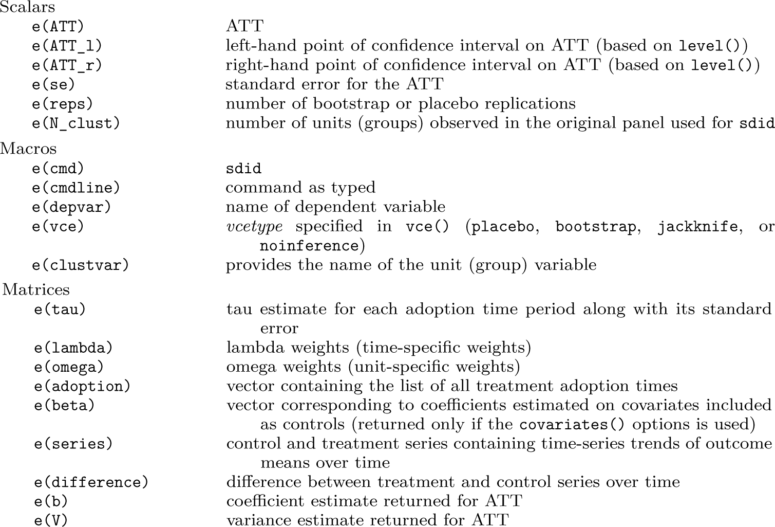
The matrices e(b) and e(V) are included to facilitate the exportation of results from sdid with commands such as estout (Jann 2004).

4 Examples based on an empirical application

In the sections below, we provide several illustrations of the usage and performance of the sdid command, which operationalizes the SDID estimator in Stata. We consider both a block treatment design (with a single adopting state) and a staggered adoption design, noting several points covering estimation, inference, and visualization.

4.1 A block design

In the first case, we consider the well-known example, also presented in Arkhangelsky et al. (2021), of California’s “Proposition 99” tobacco control measure. This example, based on the context described in Abadie, Diamond, and Hainmueller (2010) and the data of Orzechowski and Walker (2005), is frequently used to illustrate SC-style methods. Proposition 99, which was passed by California in 1989, increased the taxes paid on a pack of cigarettes by 25 cents. The impact of this reform is sought to be estimated by comparing the evolution of sales of cigarettes in packs per capita in California (the treated state) with those in 38 untreated states, which did not significantly increase cigarette taxes during the study period.

The data used in this analysis cover each of these 38 states over the period of 1970-2000, with a single observation for each state and year. Adoption occurs in California in 1989, implying T_pre = 19 pretreatment periods and T_post = 12 posttreatment periods. There are N_C0 = 38 control states and 1 treated state, so N_tr = 1. Using the sdid command, we replicate the results from Arkhangelsky et al. (2021). In the code example below, we first download the data and then conduct the SDID implementation using a placebo inference procedure with (the default) 50 placebo iterations.

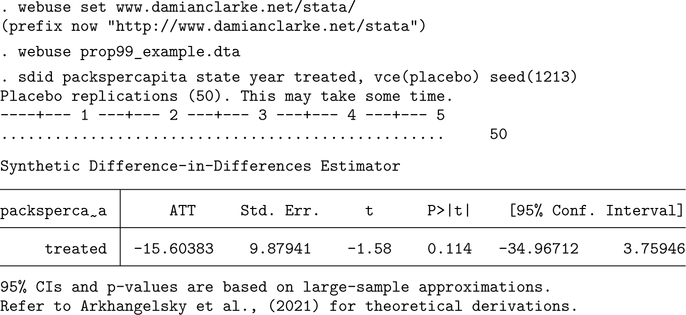
The third line of this code excerpt simply implements the SDID estimator, returning identical point estimates to those documented in table 1 of Arkhangelsky et al. (2021). Standard errors are slightly different because they are based on pseudo-random placebo reshuffling, though they can be replicated as presented here provided that the same seed is set in the seed() option. Note that in this case, given that only one treated unit is present, placebo inference is the only appropriate procedure, as specified in the vce() option.

Table 1.

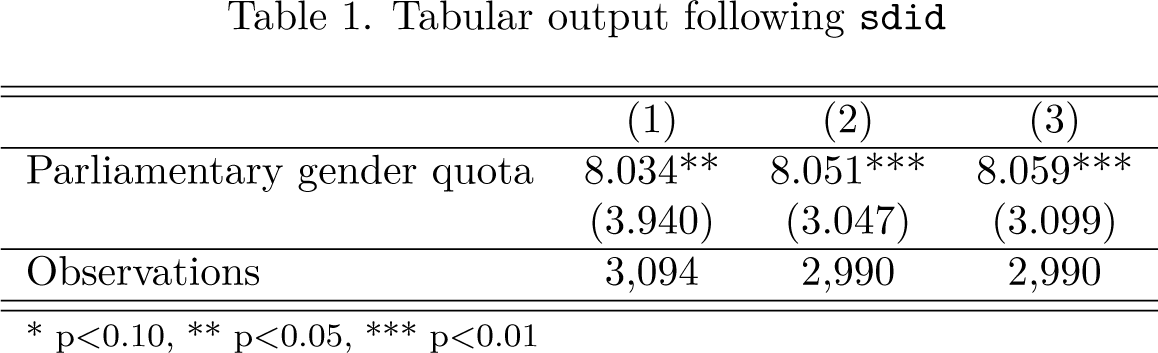
Tabular output following sdid

	(1)	(2)	(3)
Parliamentary gender quota	8.034** (3.940)	8.051*** (3.047)	8.059*** (3.099)
Observations	3,094	2,990	2,990

* p < 0.10, ** p < 0.05, *** p < 0.01

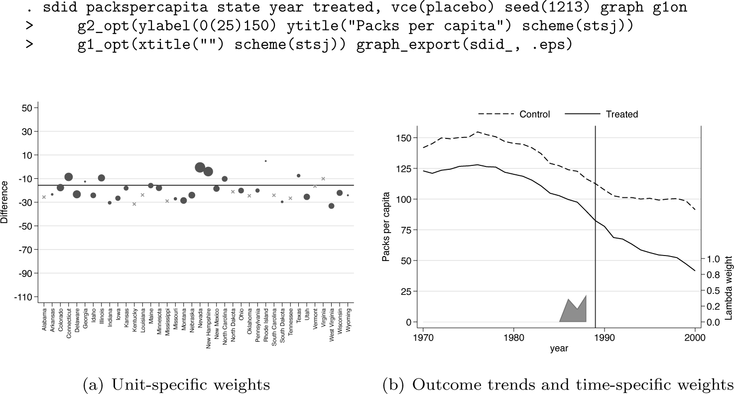
We may wish to generate the same graphs as in Arkhangelsky et al. (2021), summarizing both 1) unit-specific weights and 2) treatment and SC outcome trends along with time-specific weights. This can be requested with the graph option. This is displayed below, where we additionally modify plot aesthetics via the g1_opt() and g2_opt() options for weight graphs [figure 1(a)] and trend graphs [figure 1(b)], respectively. Finally, generated graphs can be saved to disk using the graph_export() option, with a graph type (.eps below) and optionally a prepended plot name. Output corresponding to the command below is provided in figure 1.

It is illustrative to compare the output of SDID estimation procedures with those of standard SC methods of Abadie, Diamond, and Hainmueller (2010) and unweighted DID estimates. Using the method() option, one can request a standard DID output with method(did) or an SC output with method(sc) . In the interest of completeness, method(sdid) is also accepted, although this is the default behavior when method() is not included in the command syntax. In each case, the resulting graph will match treated and control or SC trends, as well as weights received by each unit and time period. These are displayed in figure 2, with plots corresponding to each of the three calls to sdid displayed below. In the left-hand panel, identical SDID plots are provided as those noted above. In the middle plot, corresponding to method(did), a DID setting is displayed. Here, in the top panel, outcomes for California are displayed as a solid line, while mean outcomes for all control states are documented as a dashed line, where a clear divergence is observed in the pretreatment period. The bottom panel shows that in this case, each control unit receives an identical weight, while time weights indicated at the base of the top plot note that each period is weighted identically. Finally, in the case of SC, output from the third call to sdid is provided in the right-hand panel. In this case, treated and SC units are observed to overlap nearly exactly, with weights in figure 2f noted to be more sparse and placing relatively more weight on fewer control states. We note that in each case, the vce(noinference) option is used because here we are simply interested in observing exported graphs, not the entire command output displaying aggregate estimates, standard errors, and confidence intervals.

Figure 2.

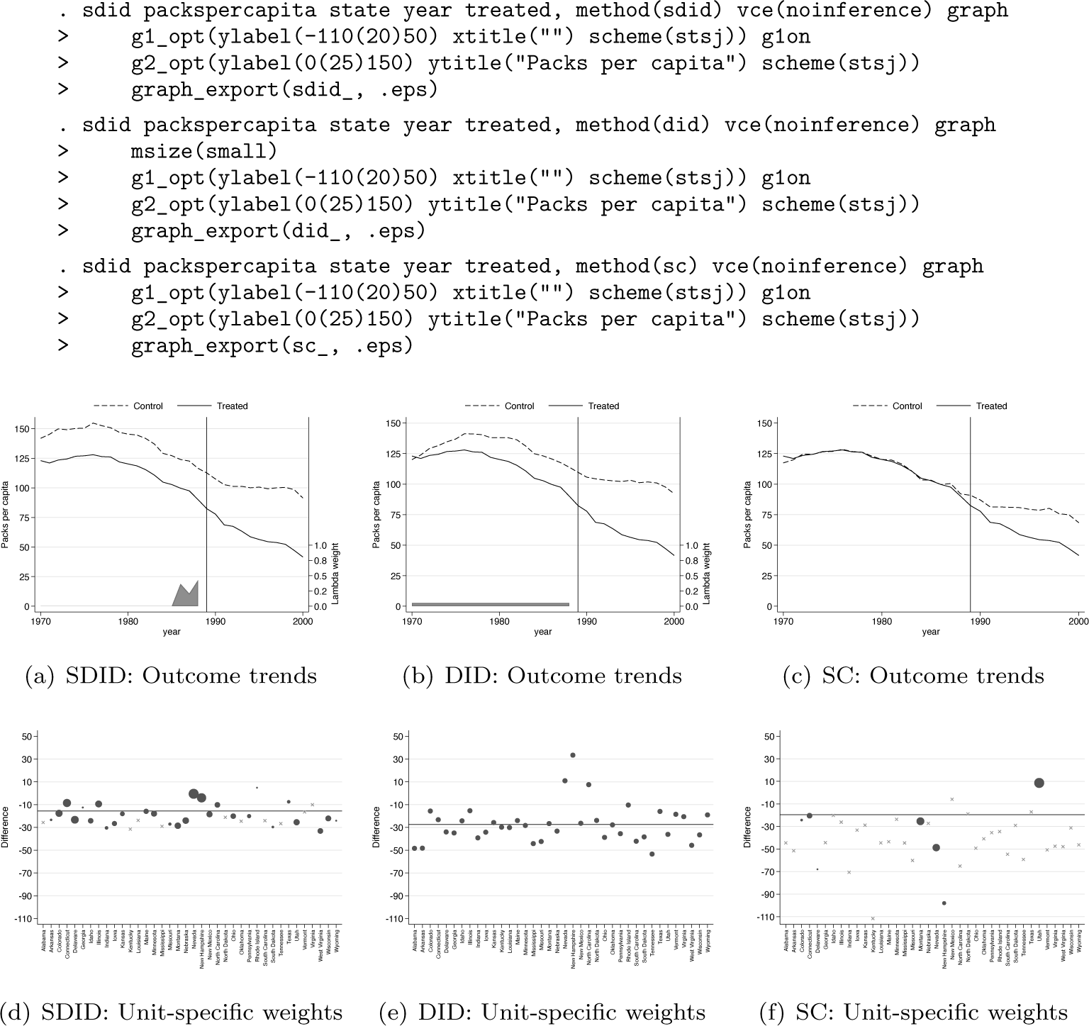
Comparison of estimators

The sdid command returns multiple matrices containing treatment and control outcome trends, weights, and other elements. These elements can be accessed for use in postestimation procedures or graphing. As a simple example, the following code excerpt accesses treatment and SC outcome trends (stored in e(series)) and time weights (stored in e(lambda)) and uses these elements to replicate the plot presented in figure 1b. The resulting graphical output is presented as figure 3, which is virtually identical to figure 1b but omits the second y axis in line with the plots originally presented in Arkhangelsky et al. (2021). In this way, if one wishes to have further control over the precise nature of plotting beyond that provided in the graphing options available in sdid’s command syntax, one can simply work with elements returned in the ereturn list command. In online appendix A2, we show that with slightly more effort, returned elements can be used to construct the unit-specific weight plot from figure 1a.

Figure 3.

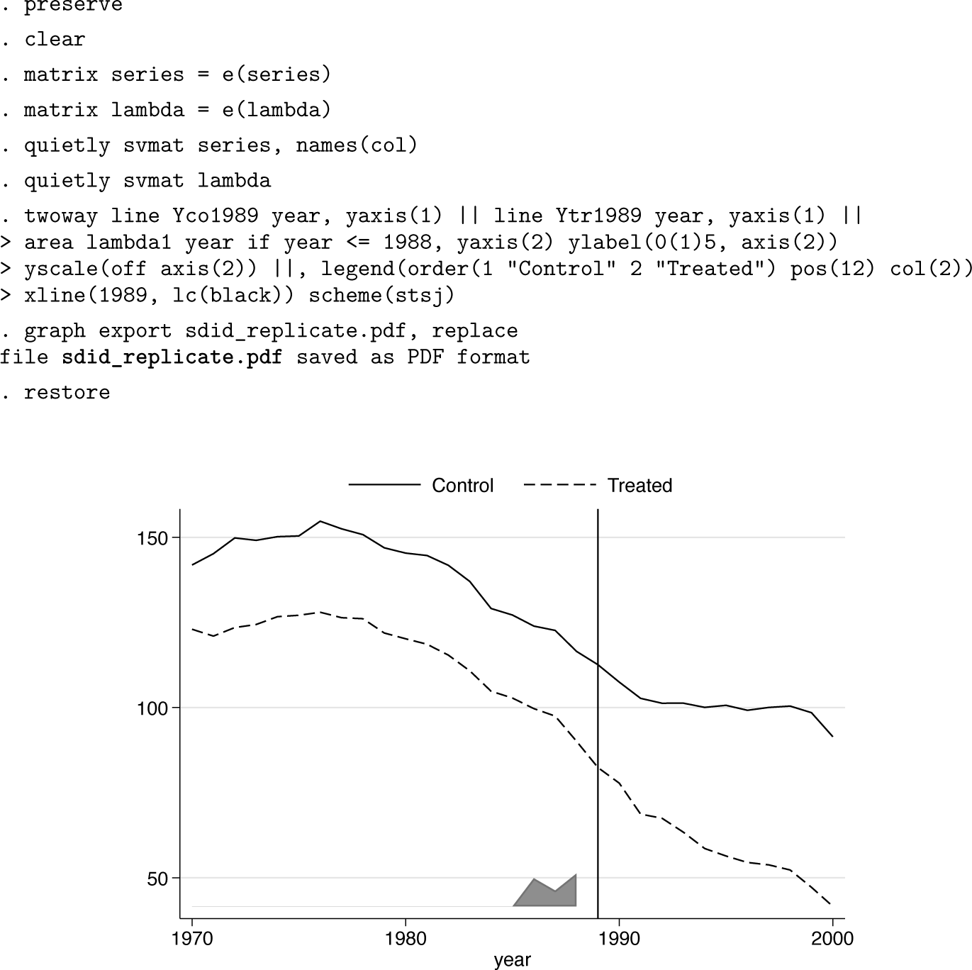
Outcome trends and time-specific weights

4.2 A staggered adoption design

We present an example of a staggered adoption design based on data and the context studied in Bhalotra et al. (2023). In this case, the impact of parliamentary gender quotas that reserve seats for women in parliament is estimated, first on rates of women in parliament and second on rates of maternal mortality. This is conducted on a country-by-year panel, where for each year of 1990-2015, 115 countries are observed, 9 of which implement a parliamentary gender quota. ⁴ For each of these countries, data on the rates of women in parliament and the maternal mortality ratio are collected, as well as several covariates.

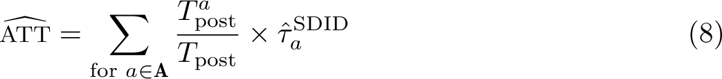
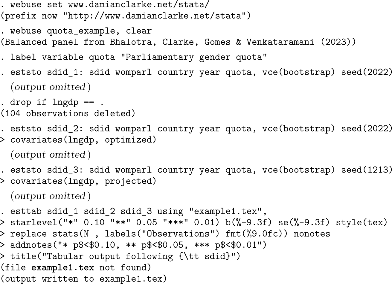
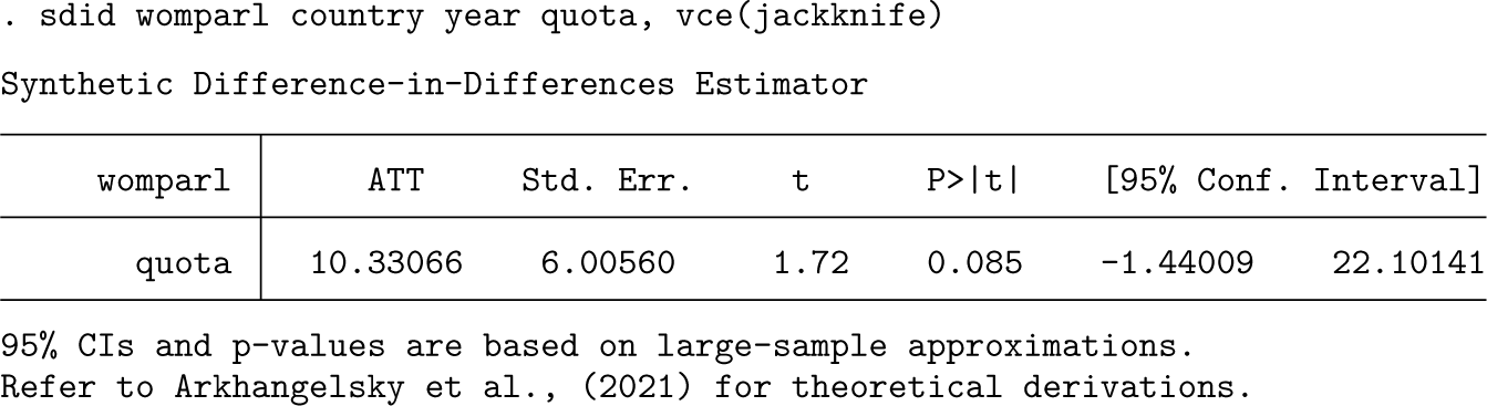
This example presents a staggered adoption configuration, given that in the period under study, quota adoption occurred in seven different yearly periods between 2000 and 2013. sdid handles a staggered adoption configuration seamlessly without any particular changes to the syntax. In the code below, we implement the SDID estimator using the bootstrap procedure to calculate standard errors. By default, the output reports the weighted ATT, which is defined in (8) above. However, as laid out in (8), this is based on each adoption-period-specific SDID estimate. These adoption-period-specific estimates are returned in the matrix e(tau), which is tabulated below the standard command output.

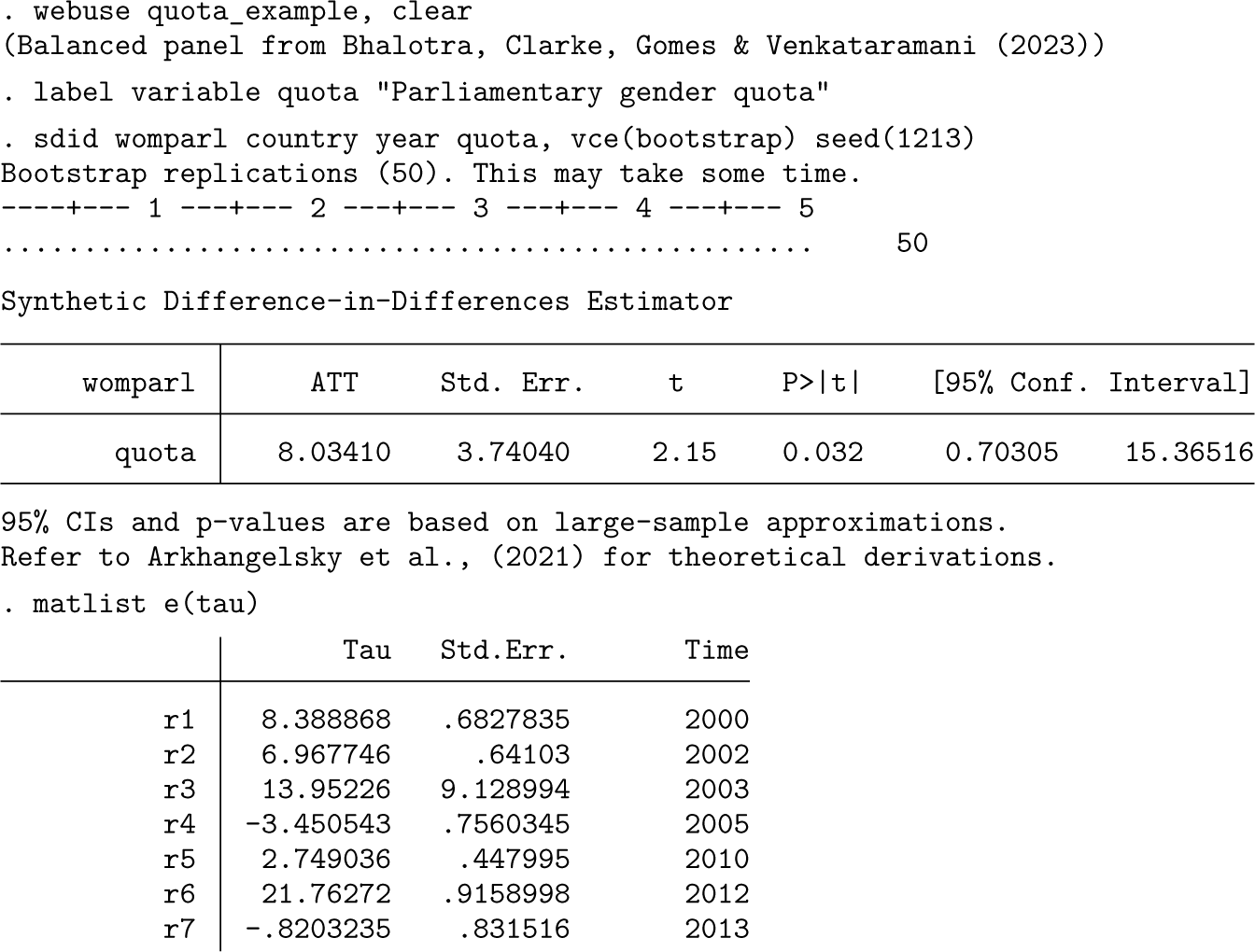
All other elements are identical to those documented in the case of a single adoption period but are generalized to multiple adoptions. For example, if one is requesting graphical output, a single treatment versus SC trend graph and corresponding unit-level weight graph is provided for each adoption date. Similarly, matrices returned with ereturn, such as e(lambda), e(omega), and e(series), provide columns for each particular adoption period.

Adding covariates. As laid out in section 2.2, covariates can be handled in SDID in several ways. Below, we document the inclusion of a single covariate (the natural logarithm of gross domestic product per capita). Because sdid is based on a balanced panel of observations, we must first ensure that there are no missing observations for all covariates, in this case dropping a few (control) countries for which this measure is not available. We then include covariates via the covariates() option. In the first case, this is conducted exactly following the procedure discussed by Arkhangelsky et al. (2021), in which parameters on covariates are estimated within the optimization routines in Mata. This is analogous to indicating covariates(, optimized). Estimates in this particular case suggest that the inclusion of this control does little to dampen effects. After estimation, the coefficients on the covariates can be inspected as part of e(beta), where an adoption-specific value for each covariate is provided, given that the underlying SDID estimate is calculated for each adoption period.

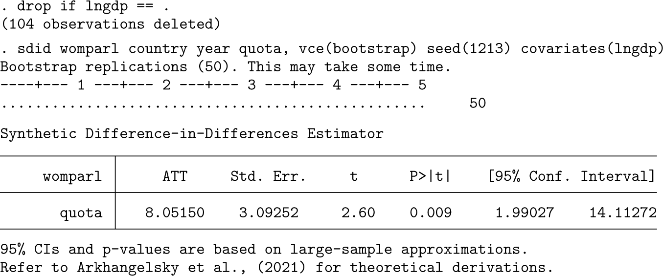
The inclusion of covariates in the previous implementation adds considerably to the computational time because it increases the complexity of the underlying optimization routine; this is conducted in each adoption period and each bootstrap replicate. An alternative way to capture covariates described in section 2.2 above is that of Kranz (2022), where the impact of covariates is projected out using a baseline regression of the outcome on covariates and fixed effects only in units where the treatment status is equal to zero. This is implemented as below with covariates(, projected).

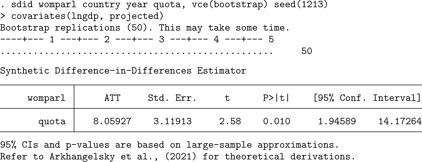
Here results are slightly different but quantitatively comparable with those when using alternative procedures for conditioning out covariates. In this case, if examining the e(beta) matrix, only a single coefficient will be provided because the regression used to estimate the coefficient vector is always based on the same sample. This additionally offers a nontrivial speedup in the execution of the code. For example, on a personal computer with Stata/SE 15.1 and relatively standard specifications, using the optimized method above required 324 seconds of computational time while using projected required 61 seconds (compared with 58 seconds where covariates were not included in sdid).

Postestimation commands. While sdid provides standard tabular and graphical outputs as displayed previously, it can be used to provide output in alternative formats. For example, the sdid command interacts seamlessly with routines such as estout for the exportation of results tables. To illustrate, the block of code below estimates three specific versions of the model discussed above, storing each model using an eststo: prefix before finally exporting estimated ATTs and standard errors to a latex file, which can be included in tabular form as displayed in table 1. Similar procedures could be conducted with routines such as outreg or outreg2, and tabular output could be further enriched using additional options within esttab if desired.

4.3 Inference options

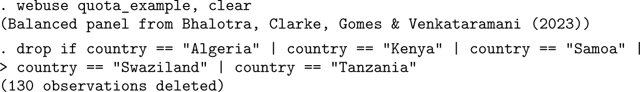
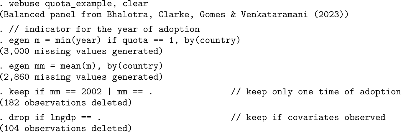
In this section, we provide examples of the implementation of alternative inference options, as laid out in algorithms 2-4. For this illustration, we will keep only treated units that adopt gender quotas in 2002 and 2003. Otherwise, adoption periods will exist in which only a single unit is treated, and jackknife procedures will not be feasible.

In the following three code blocks, we document bootstrap, placebo, and jackknife inference procedures. The difference in implementation in each case is very minor, simply indicating bootstrap, placebo, or jackknife in the vce() option. For example, for bootstrap inference, where block bootstraps over the variable country are performed, the syntax is as follows:

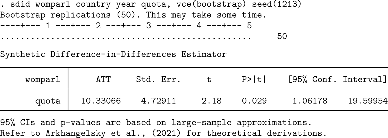
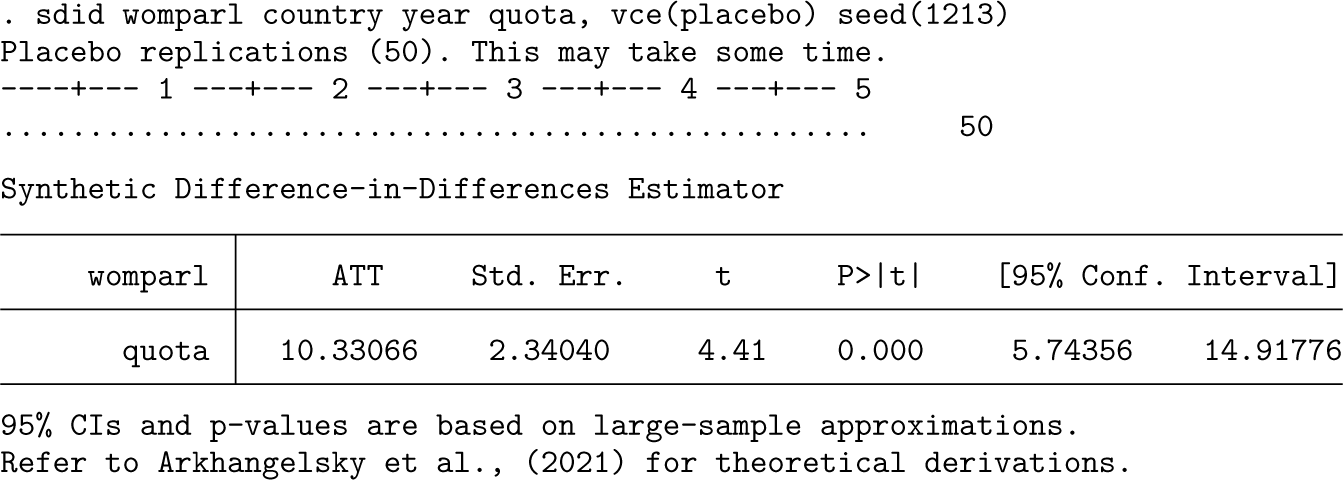
By default, only 50 bootstrap replicates are performed, though in practice, substantially more should be used; this can be specified in the reps() option. For placebo, the syntax and output are virtually identical. The suitability of each method depends on the underlying structure of the panel, and in this particular case, given the relatively small number of treated units, placebo procedures may be preferred.

Finally, in the interest of completeness, the jackknife procedure, which is by far the fastest of the three to execute,⁵ is provided below. Note that unlike the case with placebo or bootstrap inference, it is not necessary (or relevant) to set a seed or indicate the number of replications because the jackknife procedure implies conducting a leave-one-out procedure over each unit. In this particular case, jackknife inference appears to be more conservative than bootstrap procedures, in line with what may be expected based on the demonstration of Arkhangelsky et al. (2021) that jackknife inference is generally conservative.

4.4 Event-study-style output

While sdid offers a simple implementation to conduct standard SDID procedures and provide output, results can also be visualized in alternative ways with some work. For example, consider the standard “panel event-study”-style setting (see, for example, Freyaldenhoven, Hansen, and Shapiro [2019]; Schmidheiny and Siegloch [2019]; and Clarke and Tapia-Schythe [2021]), where one wishes to visualize how the dynamics of some treatment effect evolve over time, as well as how differences between treated and control units evolve prior to the adoption of treatment. Such graphs are frequently used to efficiently provide information on both the credibility of parallel pretrends in an observational setting and the emergence of any impact owing to treatment once treatment is switched on.

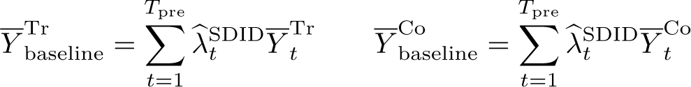
What such an analysis seeks to document is the differential evolution of treated and (synthetic) control units, abstracting away from any baseline difference between the groups. As an example, refer to figure 4a, which is based on the adoption of gender quotas laid out in section 4.2, particularly quota adoption in the year 2002. This is standard output from sdid, presenting trends in rates of women in parliament in countries that adopted quotas in 2002 (solid line) and SC countries that did not adopt quotas (dashed line). We will refer to the values plotted in these trend lines as ${\overline{Y}}_t^{\mathrm{Tr}}$ for treated units in year t and ${\overline{Y}}_t^{\mathrm{Co}}$ for SC units in year t. While this standard output allows us to visualize trends in the two groups in a simple way, it is not immediately clear how the differences in these outcomes evolve over time compared with baseline differences or with the confidence intervals on any such changes over time.

Figure 4.

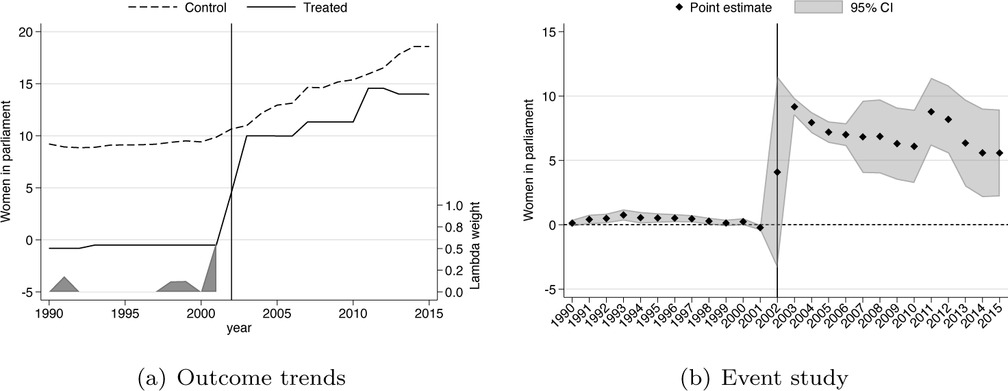
Outcome trends and event-study-style estimate of the impact of quotas on percent women in parliament

For this to resemble the logic of an event-study analysis, we wish to consider, for each period t, whether differences between treated units and SCs have changed when compared with baseline differences. Namely, for each period t, we wish to calculate

$$({\overline{Y}}_{\mathrm{t}}^{\mathrm{Tr}}-{\overline{Y}}_{\mathrm{t}}^{\mathrm{Co}})-({\overline{Y}}_{\mathrm{baseline}}^{\mathrm{Tr}}-{\overline{Y}}_{\mathrm{baseline}}^{\mathrm{Co}})(9)$$

(9)

along with the confidence interval for this quantity. Here ${\overline{Y}}_{\mathrm{baseline}}^{\mathrm{Tr}}$ and ${\overline{Y}}_{\mathrm{baseline}}^{\mathrm{Co}}$ refer to baseline (pretreatment) means for treated and SC units, respectively. In standard panel event studies, some arbitrary baseline period is chosen off of which to estimate pretreatment differences. This is often one year prior to treatment. For SDID, where pretreatment weights are optimally chosen as ${\hat{\lambda }}_t^{\mathrm{SDID}}$ (refer to section 2), this suggests an alternative quantity for ${\overline{Y}}_{\mathrm{baseline}}^{\mathrm{Tr}}$ and ${\overline{Y}}_{\mathrm{baseline}}^{\mathrm{Co}}$ , namely,

$${\overline{Y}}_{\mathrm{baseline}}^{\mathrm{Tr}}=\sum _{t=1}^{T_{\mathrm{pro}}}{\hat{\lambda }}_t^{\mathrm{SDID}}{\overline{Y}}_{\mathrm{t}}^{\mathrm{Tr}}{\overline{Y}}_{\mathrm{baseline}}^{\mathrm{Co}}=\sum _{t=1}^{T_{\mathrm{pro}}}{\hat{\lambda }}_t^{\mathrm{SDID}}{\overline{Y}}_{\mathrm{t}}^{\mathrm{Co}}$$

In other words, these baseline outcomes are simply pretreatment aggregates, where weights are determined by optimal pretreatment weights (specified by the shaded gray area in figure 4a). The event study then plots the quantities defined in (9) for each time t.

An example of such an event-study-style plot is presented in figure 4b. Here black points present the quantity indicated in (9) for each year. In this case, t ranges from 1990 to 2015. While all of these points are based on a simple implementation of sdid comparing outcomes between treated and control units following (9), confidence intervals documented in gray-shaded areas of figure 4b can be generated following the resampling or permutation procedures discussed earlier in this article. Specifically, for resampling, a block bootstrap can be conducted, and in each iteration, the quantity in (9) can be recalculated for each t. The confidence interval associated with each of these quantities can then be calculated based on its variance across many (block)-bootstrap resamples.

Figure 4b, and graphs following this principle more generally, can be generated following the use of sdid. However, by default, sdid simply provides output on trends among the treated and SC units (as displayed in figure 4a). In the code below, we lay out how one can move from these trends to the event study in panel (b). Because this procedure requires conducting the inference portion of the plot manually (unlike most other procedures involving sdid where inference is conducted automatically as part of the command), the code is somewhat more involved. Thus, we discuss the code below in several blocks, terminating with the generation of the plot displayed in figure 4b.

In the first code block, we will open the parliamentary gender quota data that we used in section 4.2 and keep the particular adoption period considered here (countries that adopted quotas in 2002), as well as untreated units:

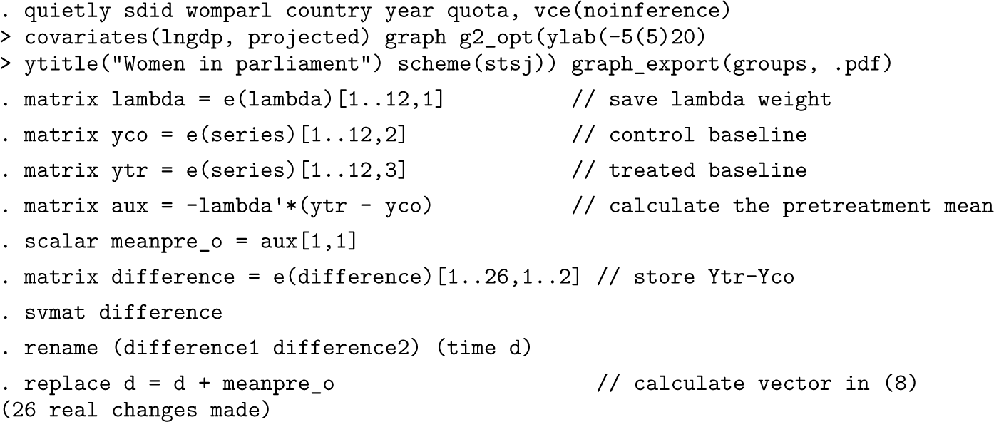
We can then implement the standard SDID procedure, additionally exporting the trend graphs, which is displayed in figure 4a. This is done in the first line below, after which several vectors are stored. These vectors allow us to calculate the quantity $({\overline{Y}}_{\mathrm{baseline}}^{\mathrm{Tr}}-{\overline{Y}}_{\mathrm{baseline}}^{\mathrm{Co}})$ indicated in (9), which is generated from ${\hat{\lambda }}_t^{\mathrm{SDID}}$ , from the returned matrix e(lambda), and pretreatment values for ${\overline{Y}}_t^{\mathrm{Tr}}$ and ${\overline{Y}}_t^{\mathrm{Co}}$ , from the returned matrix e(series). This baseline quantity is referred to as meanpre_o below. Finally, the quantity of interest in (9) for each time period t is generated as the variable d, which is plotted below as the black points on the event study in figure 4b.

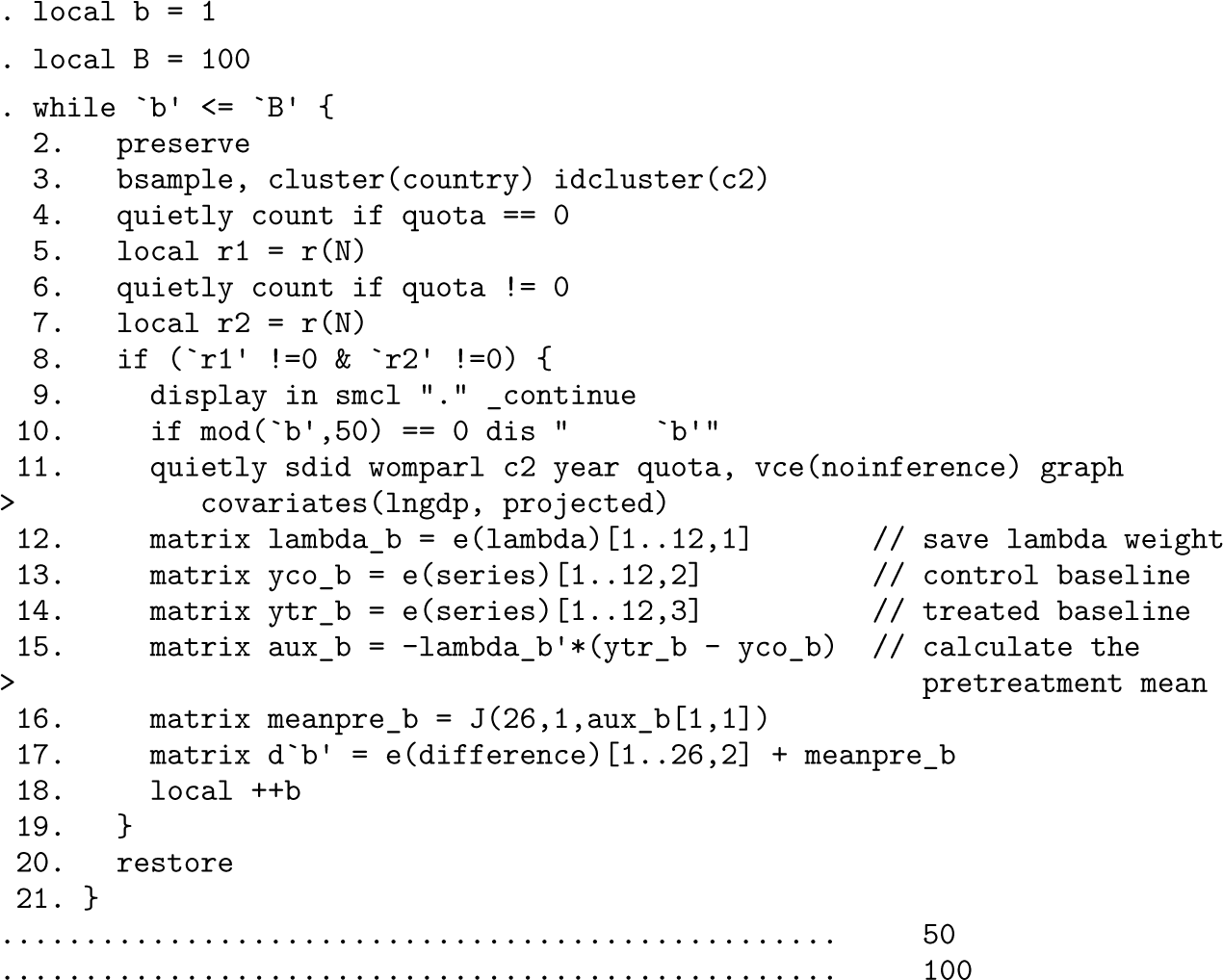
Perhaps the most complicated portion of code is that which implements the bootstrap procedure. This is provided below, where for ease of replication, we consider a relatively small number of bootstrap resamples, which is set as the local B = 100. In each bootstrap resample, we first ensure that both treatment and control units are present (using the locals r1 and r2) and then reestimate the sdid procedure with the new bootstrap sample generated using Stata’s bsample command. This is precisely the same block bootstrap procedure laid out by Arkhangelsky et al. (2021) and that sdid conducts internally. However, here we are interested in collecting, for each bootstrap resample, the same quantity estimated above with the main sample as d, which captures the estimate defined in (9) for each t. To do so, we simply follow an identical procedure as that conducted above but save the resulting resampled values of the quantities from (9) as a series of matrices d'b’ for later processing to generate confidence intervals in the event study.

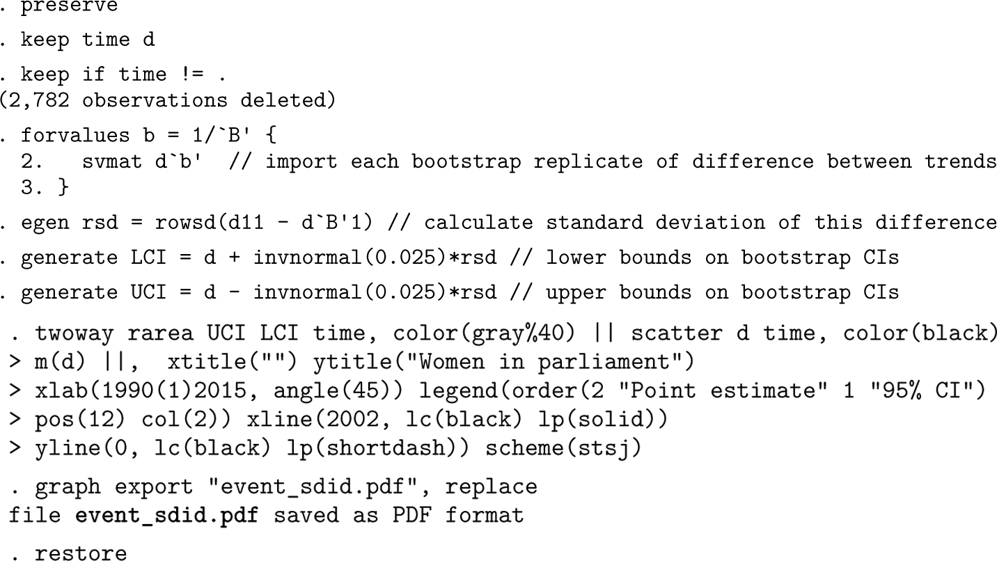
The final step is to calculate the standard deviation of each estimate from (9) based on the bootstrap resamples and then to generate confidence intervals for each parameter based on the estimates generated above (d), as well as their standard errors. This is conducted in the first lines of the code below. For each of the B = 100 resamples conducted above, we import the vector of resampled estimates from (9) and then, using rowsd(), calculate the standard deviation of the estimates across each time period t. This is the bootstrap standard error, which is used below to calculate the upper and lower bounds of 95% confidence intervals as [LCI; UCI]. Finally, based on these generated elements (d as black points on the event study and LCI and UCI as the endpoints of confidence intervals), we generate the output for figure 4b in the final lines of code.

As noted above, the outcome of this graph is provided in figure 4b, where we observe that, as expected, the SDID algorithm has resulted in quite closely matched trends between the SC and treatment group in the pretreatment period, given that all pretreatment estimates lie close to zero. The observed impact of quotas on women in parliament occurs from the treatment year onward, where these differences are observed to be large and statistically significant.

This process of estimating an event-study-style plot is conducted here for a specific adoption year. For a block adoption design where there is only one adoption period, this will be the only resulting event study to consider. However, in a staggered adoption design, a single event study could be generated for each adoption period. Potentially, such event studies could be combined, but some way would be required to deal with unbalanced lags and leads, and additionally, some weighting function would be required to group treatment lags and leads where multiple such lags and leads are available. One such procedure has been proposed in Sun and Abraham (2021) and could be a way forward here.

4.5 Other parameters

In general, estimation and inference for synthetic DID is concerned with the ATT, or adoption-specific treatment effects ${\hat{\tau }}_a^{\mathrm{SDID}}$ from (8) in the case of staggered adoption designs. Nevertheless, in considering the weighted regression model laid out in (1), we clearly see there are several other parameters involved in the estimation of the ATT, including a constant term μ, unit-fixed effects ${\alpha }_i$ , and time-fixed effects ${\beta }_t$ .

In practice, once unit- and time-specific weights are calculated, there are several ways in which one can proceed to estimate the ATT. In the implementation of sdid, given that the main estimand of interest is the ATT, a direct approach is taken where ${\hat{\tau }}^{\mathrm{SDID}}$ (or ${\hat{\tau }}_a^{\mathrm{SDID}}$ in the case of staggered adoption designs) can be estimated directly in a single weighted DID step. This procedure is laid out fully in online appendix A3, and the sdid code works in this way given that it is substantially faster in terms of total computation time than implementing the weighted regression described in (1). Nevertheless, if one wishes to estimate the other parameters associated with the objective function (1), this parameter estimation can be conducted as a postestimation step in a relatively straightforward way.

To see this, note that (1) is simply a weighted regression where weights for each unit are defined as $w={\hat{\omega }}_i^{\mathrm{SDID}}\cdot {\hat{\lambda }}_t^{\mathrm{SDID}}$ . Given that sdid returns ${\hat{\omega }}_i^{\mathrm{SDID}}$ and ${\hat{\lambda }}_t^{\mathrm{SDID}}$ as e(omega) and e(lambda) and that these results can additionally be requested to be stored directly via the returnweights option, it is illustrative to see that the weighted regression returns the parameters described in (1). We illustrate this below, taking advantage of the returnweights option in sdid.

To see how this works, we return to the case of Proposition 99, first estimating SDID. By default, when returnweights is indicated, λ weights are returned as lambda YYYY (where YYYY refers to the treatment period, which is 1989 below), and ω weights are returned as omega YYYY. If multiple treatment periods exist, a set of weights is returned for each period. In the code block below, we generate unit-specific weights implicit in sdid as weight before finally estimating the weighted regression. Output from this regression is presented below, where we observe the equivalence with the treatment effect estimated by sdid. However, we additionally observe estimated state-specific fixed effects and year-specific fixed effects, as well as the constant indicated in (1). Also, note that fixed effects exist only for those units which receive nonzero weights in the sdid algorithm. When we consider state-specific fixed effects, a single fixed effect is omitted by default (in this case, Arkansas), while all other fixed effects apart from those receiving zero weights (indicated by an “x” symbol in figure 2d) are presented in regression output. Similarly, for year-specific fixed effects, estimates exist for pretreatment years 1987 and 1988, while 1986 is omitted as the baseline reference category, in line with nonzero ω weights for these periods only.

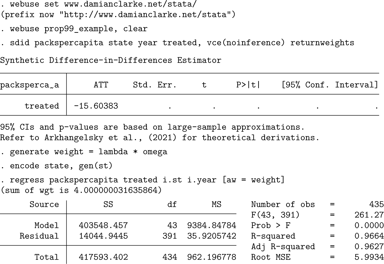
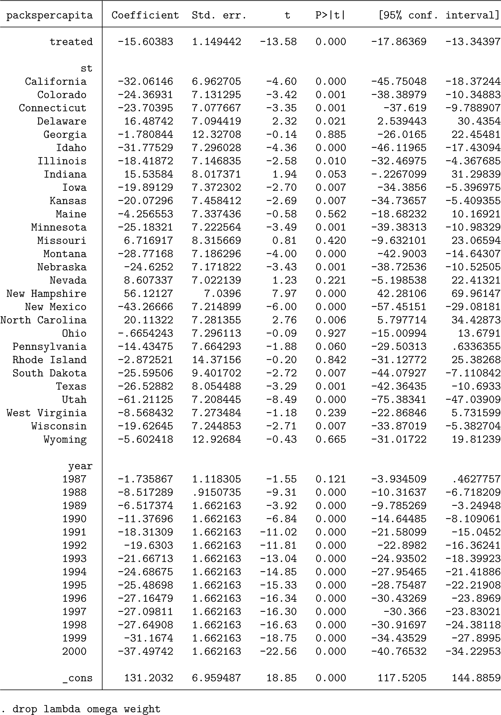
Note that this regression does not give valid inference for the estimated ATT or for any fixed effects or constants, because it treats weights as known rather than estimated. More generally, the variance derivations in Arkhangelsky et al. (2021) are valid only for the ATT, so any inference considerations on fixed effects are not theoretically founded at present. Nevertheless, if we do wish to consider valid inference in a regression-based framework following sdid, we can follow procedures similar to those laid out in the bootstrap, jackknife, or placebo procedure described previously. To consider a simple illustration, below we implement a permutation-based procedure that is virtually identical to the internal permutation routine of sdid, where in each iteration, an ATT estimate is produced for a randomly permuted (untreated) state assuming treatment occurs in 1989. We once again estimate weighted regression using the weights returned from sdid, in each iteration storing the estimated ATT in the variable Taus. Finally, at the end of this code block, we inspect estimated Taus, which provides an estimate of the standard error (the standard deviation of permutations) and similarly would allow for the calculation of confidence intervals based on empirical quantiles of this variable. We observe that the standard error is in line with that reported previously when estimating sdid directly.

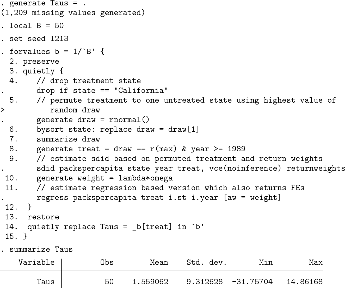
This procedure is documented because it is illustrative to note that other parameters from (1) can be simply estimated by weighted regression. Given the lack of valid standard errors directly from regression, this procedure should be implemented with care, though as we document in the permutation procedure above, one can implement valid inference directly via regression if desired, though this is less direct than implementing procedures directly in sdid. Furthermore, one could follow similar procedures to examine the variability of other parameters such as returned weights, fixed effects, or the model constant, though theoretical results are not presently available to validate the use of such procedures for valid inference on parameters apart from ${\hat{\tau }}^{\mathrm{SDID}}$ or ${\hat{\tau }}_a^{\mathrm{SDID}}$ .

5 Conclusions

Recent advances in panel-data methods have resulted in a rich set of tools that can be used to conduct policy and other analyses. Such methods, combined with a growing emphasis on formal identification and broadening availability of large datasets and computing power available to researchers (Currie, Kleven, and Zwiers 2020) suggests we will see an increasing adoption of these tools in applied research in the social sciences. Two particularly common approaches to analysis in a panel-data or repeated cross-sectional settings are DID and SC methods. While both are sharply increasing in frequency in applied research (Currie, Kleven, and Zwiers 2020), they are often used in different cases: DID is commonly employed with many treated units and potentially fewer time period, while SC is often implemented with fewer treatment units, many controls, and longer pretreatment periods. Furthermore, both settings have particular assumptions that may not be met in practice: DID requires parallel trends between treated and control units, while SC requires a convex hull assumption that is not met if treatment outcomes are more extreme than control outcomes.

In this article, we have laid out the details behind the SDID method of Arkhangelsky et al. (2021), which allows for the relaxation of assumptions required in both DID and SC settings while also maintaining desirable properties if these assumptions are met. We have discussed its implementation in Stata using the sdid command, which provides a computationally efficient way to conduct estimation, inference, and graphing. We have discussed the theory behind this command and laid out extensions into a staggered adoption setting. We provided two empirical examples to demonstrate the usage of the command. While the main novelty of the sdid command introduced here is the implementation of SDID methods, it can similarly be used to implement DID and SC methods. The efficiency of estimation routines implemented for SDID are leveraged when estimating SC and DID methods, which implies that sdid may provide faster implementations than other SC libraries currently available in Stata in a range of contexts.

Nevertheless, despite the ease of implementation of sdid, there are several requirements that should be considered prior to usage. From a practical standpoint, given the nature of the SDID algorithm, some conditions must be met for it to be applied to data. First, and most importantly, a balanced panel of data is required that provides outcomes and treatment measures for each unit in all periods under study. Should missing values in such outcomes be present in the panel, either the missing values must be eliminated from the estimation sample or data should be sought to fill in gaps (a similar requirement exists for control variables if controls are to be included in estimation). Second, no units can be considered if they were exposed to treatment from the first period in which data are observed. If this occurs, there is no pretreatment period on which to generate SC cohorts. If always-treated units are present in the data, either the units must be eliminated or earlier data must be sought. Third, pure control units are required. At least some units must never be treated to act as donor units. If all units are treated at some point in the panel, no donor units exist and SCs cannot be generated. Finally, in the case of inference, additional requirements must be met. In the case of a bootstrap or jackknife procedure, the number of treated units should be larger than one (and ideally considerably larger than this). Should only one treated unit be present, placebo inference should be conducted. Note that placebo inference can be conducted only if the number of control units exceeds the number of treated units. If one is implementing DID or SC methods using sdid, these procedures rely on similar computational routines and so inherit the same requirements mentioned above (though they also inherit the same computational efficiencies built into SDID implementations).

From a theoretical standpoint, there are additional considerations that are important to keep in mind for the implementation of SDID procedures. In particular, note that normality results underlying the generation of variance estimates and confidence intervals hold asymptotically. Specifically, these results require that the entire panel size grow without limit, as well as the number of control units and the number of pretreatment periods. However, these results do not require for the number of treatment units to grow without limit; they require that either the number of posttreatment periods or the number of treated units grows without limit (see Arkhangelsky et al. [2021, 4016]). Reassuringly, simulation results from Arkhangelsky et al. (2021) suggest the SDID estimator has good properties even with as few as one treatment unit and with panels consisting of 50 states and 40 time periods. This raises the general question of what types of data properties are required for SDID estimation. A key element of estimation, as in the case of SC estimation (Ben-Michael, Feller, and Rothstein 2021; Abadie, Diamond, and Hainmueller 2010), is the adequate modeling of pretreatment trends. This requires a sufficient number of periods off of which to model the generation of synthetic cohorts but also the avoidance of periods in which structural breaks occur in treatment outcomes (see, for example, practical discussion related to SCs in Abadie [2021]). While there is not yet a method to determine the precise number of required pretreatment periods for SDID modeling, simulation results in Arkhangelsky et al. (2021) show good behavior in settings with 30 pretreatment periods. In practice, considerably fewer pretreatments are likely to be required, and indeed, the canonical example of SC methods based on California’s Proposition 99 is based on 19 pretreatment periods. Additionally, SDID generally requires fewer pretreatment periods than SC implementations given that SDID’s optimal weighting of years and states in generating estimates has a double robustness property, while SC does not have this property (Arkhangelsky et al. 2021). Future work could further clarify data requirements in terms of minimum required preperiods in SDID modeling.

In general, this is a quickly evolving field (Roth et al. 2022; Arkhangelsky and Imbens 2023), and there is substantial work of interest beyond the synthetic DID methods described in this article. Among other things, SC has been shown to gain from regularization (Ben-Michael, Feller, and Rothstein [2021]; Chernozhukov, Wüthrich, and Zhu [2021]; and Abadie and L’Hour [2021], among others), debiasing methods (Ferman and Pinto 2021), and distributional considerations (Gunsilius 2023). Overall, though, should a balanced panel of data be available, the SDID method and the sdid command described here offer flexible, easy-to-implement, and robust options for the analysis of impacts of policies or treatments in certain groups at certain times. These methods provide clear graphical results to describe outcomes and an explicit description of how counterfactual outcomes are inferred. These methods are likely well suited to a large body of empirical work in social sciences, where treatment assignment is not random, and offer benefits over both DID and SC methods.

Supplemental Material

sj-pdf-1-stj-10.1177_1536867X241297914 - Supplemental material for On synthetic difference-in-differences and related estimation methods in Stata

Supplemental material, sj-pdf-1-stj-10.1177_1536867X241297914 for On synthetic difference-in-differences and related estimation methods in Stata by Damian Clarke, Daniel Pailañir, Susan Athey and Guido Imbens in The Stata Journal