Ordinary least squares and instrumental-variables estimators for any outcome and heterogeneity

Abstract

Given an exogenous treatment d and covariates x, an ordinary least-squares (OLS) estimator is often applied with a noncontinuous outcome y to find the effect of d, despite the fact that the OLS linear model is invalid. Also, when d is endogenous with an instrument z, an instrumental-variables estimator (IVE) is often applied, again despite the invalid linear model. Furthermore, the treatment effect is likely to be heterogeneous, say, µ₁(x), not a constant as assumed in most linear models. Given these problems, the question is then what kind of effect the OLS and IVE actually estimate. Under some restrictive conditions such as a “saturated model”, the estimated effect is known to be a weighted average, say, E{ω(x)µ₁(x)}, but in general, OLS and the IVE applied to linear models with a noncontinuous outcome or heterogeneous effect fail to yield a weighted average of heterogeneous treatment effects. Recently, however, it has been found that E{ω(x)µ₁(x)} can be estimated by OLS and the IVE without those restrictive conditions if the “propensity-score residual” d − E(d| x) or the “instrument-score residual” z−E(z| x) is used. In this article, we review this recent development and provide a command for OLS and the IVE with the propensity- and instrument-score residuals, which are applicable to any outcome and any heterogeneous effect.

1 Introduction

Given an exogenous binary treatment d, an outcome y, and covariates x, consider the ordinary least-squares (OLS) estimator of y on (x , d) for a linear model $y={\beta }_x^{\prime }x+\hspace{0.17em}{\beta }_{d}d+\text{ error}$ , where β _x and β_d are parameters. In reality, the treatment effect may not be a constant (β_d ), as is assumed in the linear model, but an unknown heterogeneous function, say, µ₁(x), that results in µ₁(x)d instead of β_dd. This is clear if one thinks of the COVID-19 vaccine effects, which can be highly heterogeneous; some individuals suffer from extremely negative effects (that is, death), while others benefit from fully positive effects. It is sometimes possible to account for µ₁(x) using interaction terms d x, but approximating µ₁(x) with d x would generally be inadequate. Hence, an important question arises: What kind of effect does the OLS slope of d estimate when the true effect is an unknown function µ₁(x) of x?

An answer is that the OLS d-slope is consistent for a Var(d| x)-weighted average of µ₁(x), where Var(d| x) denotes the variance of d conditional on x (Angrist 1998; Angrist and Krueger 1999; Angrist and Pischke 2009; and Aronow and Samii 2016). Unfortunately, however, this answer requires that E(d| x) be the same as the linear projection L(d| x), that is, the “population OLS predictor” of d using x.

Because E(d| x) = L(d| x) hardly holds in reality unless the model is saturated (that is, x is discrete, and a full set of dummy variables is used for all possible values of x), another question emerges: What effect does the OLS d-slope estimate under E(d| x) ≠ L(d| x), when the true effect is µ₁(x)? In addition to this effect-heterogeneity problem, y is often a limited dependent variable (LDV) for which the linear model does not hold in general. This raises yet another question: What effect does the OLS d-slope estimate under E(d| x) ≠ L(d| x), when the true effect is µ₁(x) or y is an LDV?

Going one step further, when d is endogenous with a binary instrument z, an instrumental-variables estimator (IVE) is often applied to an LDV y. Then an analogous question emerges: What effect does the IVE d-slope estimate under E(d| x) ≠ L(d| x), when the true effect is µ₁(x) or y is an LDV? Instead of simply raising the “passive” or “negative” questions on the (biased) estimands of OLS and the IVE in difficult situations, a more “active” or “positive” question might be, Is there any way to do a valid OLS or IVE without E(d| x) = L(d| x) to estimate a meaningful treatment effect when the true effect is µ₁(x) or y is an LDV?

This article reviews the answers to the above questions as presented in Lee (2018, 2021) and Lee, Lee, and Choi (Forthcoming) and provides the command psr, which implements the positive approaches in Lee (2018) for OLS and Lee (2021) for the IVE. In essence, the approaches are that modified versions of OLS and the IVE are consistent for some specific weighted averages of µ₁(x) for any form of y. The generality of the approaches is that they allow for an arbitrary µ₁(x) and an arbitrary form of y, either of which would invalidate the usual linear model.

The approach by Lee (2018, 2021) is related to, but more generally applicable than, that of Angrist (2001), who advocates declaring the effect of interest first and then finding ways to identify and estimate it—a point also made by van der Laan and Rose (2011) later in the name “targeted learning”. Angrist (2001) argues that simple linear estimators such as the IVE can be appropriately used even with noncontinuous outcome variables. However, such linear model estimators may exhibit bias unless E(d| x) = L(d| x), which hardly holds for general nonsaturated models. Lee, Lee, and Choi (Forthcoming) derive the bias in the context of linear probability models. Though Angrist (2001, 10) mentions the use of nonlinear least squares as a solution for LDVs, the implementation is practically inconvenient and often challenging because it may involve nuisance infinite weights. Readers are referred to the comments by Moffitt (2001), Imbens (2001), and Todd (2001) for other concerns.

In contrast, the approach by Lee (2018, 2021) presented below yields estimators that are always a weighted average of heterogeneous treatment effects, regardless of whether E(d| x) = L(d| x). Furthermore, their approach is applicable to any form of y and is straightforward to implement because it involves only linear regressions (for OLS and IVE) and widely used probit or logit.

In the remainder of this article, section 2 closely examines the above questions and answers in Lee (2018, 2021) and Lee, Lee, and Choi (Forthcoming). Section 3 presents the command psr, which performs the modified OLS and IVE for any y (continuous, binary, count, etc.) and estimates weighted averages of µ₁(x). Section 4 provides two empirical illustrations. Finally, section 5 concludes this article.

2 OLS and IVE valid for any outcome

2.1 Effect estimated by OLS

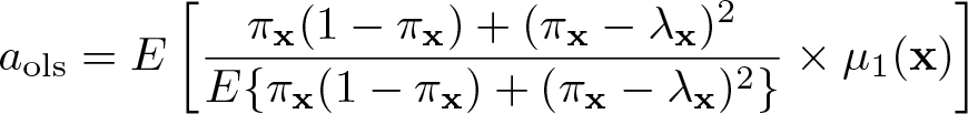
For the heterogeneous effect, µ₁(x) ≡ E(y ¹ − y ⁰ | x), where y ¹ and y ⁰ are the potential outcomes, Angrist and Pischke (2009, eq. 3.3.7) show that the slope estimator ${\widehat{\beta }}_d$ of d in the OLS regression of y on (x , d) is consistent for the weighted average

$E\left\{\omega (x){\mu }_1(x)\right\},\hspace{0.17em}\omega (x)\equiv \frac{\mathrm{Var}(d\mid x)}{E\{\mathrm{Var}(d\mid x)\}}=\frac{{\pi }_x\left(1-{\pi }_x\right)}{E\left\{{\pi }_x\left(1-{\pi }_x\right)\right\}},\hspace{1em}{\pi }_x\equiv E(d\mid x)$

1

if π _x = λ _x ≡ L(d| x) ≡ L(d x ′){E(xx ′)} ^{− 1} x, where π _x is the propensity score (PS) and Var(d| x) is the variance of d conditional on x.

The quadratic function π _x (1 − π _x ) reaches its maximum at π _x = 0.5 and its minimum at π _x = 0, 1. Considering the popular “PS matching” targeting for E{E(y ¹ − y ⁰ |π _x )}, because those subjects with π _x ≃ 0.5 overlap well with subjects in the opposite group, whereas those with π _x ≃ 0, 1 do not, Li, Morgan, and Zaslavsky (2018) called ω(x) the overlap weight (OW). That is, those subjects close to being randomized receive high weights in OW (Thomas, Li, and Pencina 2020). PS matching avoids the poor overlap problem by removing those with π _x ≃ 0, 1, which amounts to targeting for E{ω_uni(x)E(y ¹ − y ⁰ |π _x )}, where ω_uni(x) is a step-shaped “uniform weight” equal to 0 for π _x ≃ 0, 1 and a positive constant otherwise. In this context, OW ω(x) can be viewed as a smoothed version of ω_uni(x).

Using E{ω(x)µ₁(x)} instead of E{µ₁(x)} as one marginal effect accords many benefits in causal analysis, such as 1) stabilizing “inverse probability weighting” estimators (Li and Greene 2013), 2) making “regression adjustment/imputation” estimators robust to misspecified outcome regression models (Vansteelandt and Daniel 2014), and 3) automatically ensuring the exact covariate balance when π _x is logistic (Li, Morgan, and Zaslavsky 2018). More advantages of OW can be seen in Choi and Lee (2023), who provide a review on OW.

OW is far more pervasive in the statistical, medical, and epidemiological literature than most researchers are aware. In recent years, in addition to the studies mentioned above, there appeared many studies advocating OW: Mao et al. (2018), Mao, Li, and Greene (2019), Li and Li (2019), Li, Thomas, and Li (2019), Mlcoch et al. (2019), Mao and Li (2020), and Cheng et al. (2022), among others. Bear in mind that OW ω(x) is not something artificial, because it is a smooth version of ω_uni(x) and it appears naturally in partialing out ${\beta }_{\text{x}}^{\prime }x$ in $y={\beta }_x^{\prime }x+{\mu }_1(x)d+\text{error}$ .

Turning back to the Angrist and Pischke (2009) derivation, we see the convergence of the OLS estimator to the weighted average in (1) requires restrictively π _x = λ _x , where λ _x is the linear projection of d on x as defined above. To ensure π _x = λ _x , Angrist and Pischke (2009) assume a saturated model, but saturated models are rare.

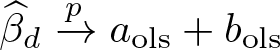
In general, π _x ≠ λ _x (for example, probit for π _x ) and the OLS slope estimator may not converge to a weighted average of µ₁(x). For example, for binary y, Lee, Lee, and Choi (Forthcoming) show that

${\widehat{\beta }}_d\stackrel{p}{\to }{a}_{\text{ols}}+\hspace{0.17em}{b}_{\text{ols}}$

where ${\widehat{\beta }}_d$ is the OLS d-slope estimator,

$a_{\text{ols}}=E\left[\frac{{\pi }_x\left(1-{\pi }_x\right)\hspace{0.17em}+\hspace{0.17em}{\left({\pi }_x-{\text{λ}}_x\right)}^2}{E\left\{{\pi }_x\left(1-{\pi }_x\right)\hspace{0.17em}+\hspace{0.17em}{\left({\pi }_x-{\text{λ}}_x\right)}^2\right\}}\hspace{0.17em}\times \hspace{0.17em}{\mu }_1(x)\right]$

is a weighted average of µ₁(x), and b_ols is a bias term. If π _x = λ _x , a_ols reduces to E{ω(x)µ₁(x)} in (1) and b_ols = 0. Otherwise, a_ols + b_ols is hard to interpret. The weighting function in a_ols makes little sense if π _x ≠ λ _x , and the bias term b_ols involves E(y ⁰ | x) and µ₁(x) (see Lee, Lee, and Choi [Forthcoming, eq. 11]) for the exact formula of b_ols. In contrast, the methods proposed by Lee (2018, 2021) presented in the following sections always yield estimators that are consistent for a specific weighted average of treatment effects for any outcome and heterogeneity.

2.2 OLS with PS residual

For exogenous d, Lee (2018) shows that the OLS of y on d − π _x is consistent for E{ω(x)µ₁(x)} for any form of y regardless of whether π _x = λ _x , as long as y ¹ − y ⁰ makes sense. y ¹ − y ⁰ makes sense for continuous, count, or binary y; for categorical y, turn each category to a dummy variable to use each dummy variable as an outcome. In fact, Lee’s (2018) OLS was suggested much earlier by Robins, Mark, and Newey (1992) for a constant-effect semilinear model y = µ₀(x) + β_dd + error with a continuous y and an unknown function µ₀(x).

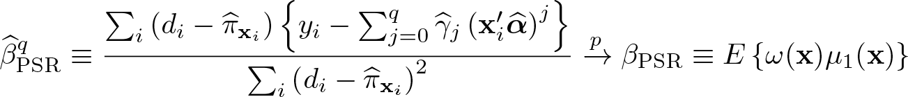
Although π _x can be estimated nonparametrically, to make the OLS practical, Lee (2018) uses the probit π _x and proposed the OLS of y − E(y|π _x ) on d − π _x . Using y − E(y|π _x ) instead of y makes the OLS robust to misspecifications in π _x to the extent that the OLS of y − E(y|π _x ) on d − π _x is close to the OLS of y − E(y| x) on d − π _x , which is “double debiased/orthogonalized” (Chernozhukov et al. 2017, 2018, 2022). Denote the OLS of y − E(y|π _x ) on the PS residual (PSR) d − π _x “OLS_PSR”, and denote the OLS as “ ${\widehat{\beta }}_{\text{PSR}}^q$ ”; q in ${\widehat{\beta }}_{\text{PSR}}^q$ is explained shortly.

To implement OLS_PSR, 1) obtain the probit of d on x to get the estimator ${\widehat{\pi }}_x\hspace{0.17em}\equiv \hspace{0.17em}\Phi \left(x^{\prime }\widehat{\alpha }\right)$ , where Φ(·) is the standard normal distribution function and x ′ α is the probit regression function with a parameter α , 2) obtain the OLS $\left({\widehat{\gamma }}_0,\hspace{0.17em}\dots ,\hspace{0.17em}{\widehat{\gamma }}_q\right)$ of y on $\left\{{\left(x^{\prime }\widehat{\alpha }\right)}^0,\hspace{0.17em}\dots ,\hspace{0.17em}{\left(x^{\prime }\widehat{\alpha }\right)}^q\right\}$ to get the predicted value ${\displaystyle {\sum }_{j=0}^q\hspace{0.17em}{\widehat{\gamma }}_j}{\left(x^{\prime }\widehat{\alpha }\right)}^j$ for E(y|π _x )—Lee (2018) suggested q = 2 or 3—and 3) do the OLS of $y\hspace{0.17em}-\hspace{0.17em}{\displaystyle {\sum }_{j=0}^q\hspace{0.17em}{\widehat{\gamma }}_j}{\left(x^{\prime }\widehat{\alpha }\right)}^j$ on $d-{\widehat{\pi }}_x$ :

${\widehat{\beta }}_{\text{PSR}}^q\hspace{0.17em}\equiv \hspace{0.17em}\frac{{\displaystyle {\sum }_i\left(d_i\hspace{0.17em}-\hspace{0.17em}{\widehat{\pi }}_{x_i}\right)\hspace{0.17em}\left\{y_i\hspace{0.17em}-\hspace{0.17em}{\displaystyle {\sum }_{j=0}^q\hspace{0.17em}{\widehat{\gamma }}_j}{\left({x^{\prime }}_i\widehat{\alpha }\right)}^j\right\}}}{{\displaystyle {\sum }_i{\left(d_i\hspace{0.17em}-\hspace{0.17em}{\widehat{\pi }}_{x_i}\right)}^2}}\hspace{0.17em}\stackrel{p}{\to }\hspace{0.17em}{\beta }_{\text{PSR}}\hspace{0.17em}\equiv \hspace{0.17em}E\left\{\omega (x){\mu }_1(x)\right\}$

Because Φ(·) is one to one, E(y|π _x ) = E(y| x ′ α ) holds, which implies that step 2 above can be done equivalently by the OLS regression of y on the polynomials of the predicted probability ${\widehat{\pi }}_x$ instead of the linear index $x^{\prime }\widehat{\alpha }$ . Although using $x^{\prime }\widehat{\alpha }$ and using ${\widehat{\pi }}_x$ are theoretically equivalent, they can differ in practice. On one hand, if there are outliers in $x^{\prime }\widehat{\alpha }$ , then it is better to use ${\widehat{\pi }}_x$ because the outlier problem would be more subdued in ${\widehat{\pi }}_x$ . On the other hand, if ${\widehat{\pi }}_x$ is too small, then ${\widehat{\pi }}_X^2$ and ${\widehat{\pi }}_X^3$ would be almost zero, in which case it is better to use $x^{\prime }\widehat{\alpha }$ .

For some Ω_ols and an independent and identically distributed sample of size n, we have $\sqrt{n}\left({\widehat{\beta }}_{\text{PSR}}^q\hspace{0.17em}-\hspace{0.17em}{\beta }_{\text{PSR}}\right)\hspace{0.17em}\stackrel{d}{\to }\hspace{0.17em}N\left(0,\hspace{0.17em}{\Omega }_{\text{ols}}\right)$ ,

$\begin{array}{l}{\widehat{\Omega }}_{\text{ols}}\hspace{0.17em}\equiv \hspace{0.17em}{\left(\frac{1}{n}\hspace{0.17em}{\displaystyle \sum _i{\widehat{\epsilon }}_i^2}\right)}^{-2}\hspace{0.17em}\cdot \hspace{0.17em}\frac{1}{n}\hspace{0.17em}{\displaystyle \sum _i{\left({\widehat{v}}_i{\widehat{\epsilon }}_i\hspace{0.17em}+\hspace{0.17em}\widehat{{\mathcal{l}}^{\prime }}{\widehat{\eta }}_i\right)}^2}\hspace{0.17em}\stackrel{p}{\to }\hspace{0.17em}{\Omega }_{\text{ols}}\\ {\widehat{\epsilon }}_i\hspace{0.17em}\equiv \hspace{0.17em}{d}_i\hspace{0.17em}-\hspace{0.17em}\Phi \left({x^{\prime }}_i\widehat{\alpha }\right),\hspace{1em}{\widehat{v}}_i\hspace{0.17em}\equiv \hspace{0.17em}{y}_i\hspace{0.17em}-\hspace{0.17em}{\displaystyle \sum _{j=0}^q\hspace{0.17em}{\widehat{\gamma }}_j}\left({x^{\prime }}_i\widehat{\alpha }\right){\hspace{0.17em}}^j\hspace{0.17em}-\hspace{0.17em}{\widehat{\beta }}_{\text{psr}}^q{\widehat{\epsilon }}_i,\\ \widehat{\mathcal{l}}\hspace{0.17em}\equiv \hspace{0.17em}-\frac{1}{n}\hspace{0.17em}{\displaystyle \sum _i{x}_i}{\widehat{v}}_i\varphi \left({x^{\prime }}_i\widehat{\alpha }\right),\hspace{1em}{\widehat{\eta }}_i{ }_i\hspace{0.17em}\equiv \hspace{0.17em}{\left(\frac{1}{n}{\displaystyle \sum _i{\widehat{s}}_i}{{\widehat{s}}^{\prime }}_i\right)}^{-1}{\widehat{s}}_i,\hspace{1em}{\widehat{s}}_i\hspace{0.17em}\equiv \hspace{0.17em}\frac{{\widehat{\epsilon }}_i\varphi \left({x^{\prime }}_i\widehat{\alpha }\right)}{\Phi \left({x^{\prime }}_i\widehat{\alpha }\right)\left\{1\hspace{0.17em}-\hspace{0.17em}\Phi \left({x^{\prime }}_i\widehat{\alpha }\right)\right\}}{x}_i\end{array}$

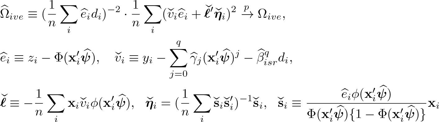
The probit score function ${\widehat{s}}_i$ involves h(t) ≡ ϕ(t)/[Φ(t){1 − Φ(t)}], which can be difficult to evaluate numerically when |t| is large. In our experiments, h(t) seems difficult to obtain precisely when t < −20 or t > 5. Hence, using the symmetry of h(t), we compute h(t) by h(−|t|) so that h(t) can be found reliably for |t| < 20. For extreme t values outside the range |t| > 20, using h(t)/|t| → 1 as |t| → ∞, we replace h(t) with |t|. If logit were used for π _x , then this kind of numerical problem would not appear, because the part in logit corresponding to h(t) is equal to 1.

2.3 IVE with instrument-score residual

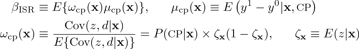
Generalizing Lee (2018), Lee (2021) allowed d to be endogenous with a binary instrument z. Defining the “instrument score” (IS) ζ _x ≡ E(z| x), Lee (2021) proposed the IVE of y − E(y|ζ _x ) on d with the IS residual (ISR) z − ζ _x as the instrument.

Let (d ⁰ , d ¹) be the potential treatments of d for z = 0, 1, and define “compliers” (CPs) as those with d ⁰ = 0 and d ¹ = 1. The IVE, dubbed “IVE_ISR”, is consistent for

$\begin{array}{l}{\beta }_{\text{ISR}}\hspace{0.17em}\equiv \hspace{0.17em}E\left\{{\omega }_{\text{cp}}(x){\mu }_{\text{cp}}(x)\right\},\hspace{1em}{\mu }_{\text{cp}}(x)\hspace{0.17em}\equiv \hspace{0.17em}E\left(y^1\hspace{0.17em}-\hspace{0.17em}{y}^0\mid x,\hspace{0.17em}\text{CP}\right)\\ {\omega }_{\text{cp}}(x)\hspace{0.17em}\equiv \hspace{0.17em}\frac{\mathrm{Cov}(z,\hspace{0.17em}d\mid x)}{E\{\mathrm{Cov}(z,\hspace{0.17em}d\mid x)\}}\hspace{0.17em}=\hspace{0.17em}P(\text{CP}\mid x)\hspace{0.17em}\times \hspace{0.17em}{\zeta }_x\left(1\hspace{0.17em}-\hspace{0.17em}{\zeta }_x\right),\hspace{1em}{\zeta }_x\hspace{0.17em}\equiv \hspace{0.17em}E(z\mid x)\end{array}$

The weight is high for subjects with a high Cov(z, d| x), avoiding the “weak instrument problem” in the IVE. More importantly, the weight becomes an OW when z is taken as the underlying treatment, as in the “intent-to-treat effect” in clinical trials with an assignment z and the actual (not well complied) treatment d. Note that β_ISR becomes E{ω(x)µ₁(x)} for exogenous d because then d = z and everybody is a complier.

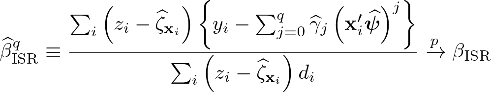
To implement IVE_ISR, 1) obtain the probit of z on x to get the estimator ${\widehat{\zeta }}_x\hspace{0.17em}\equiv \hspace{0.17em}\Phi \left(x^{\prime }\widehat{\psi }\right)$ for ζ _x ; 2) obtain the OLS $\left({\widehat{\gamma }}_0,\hspace{0.17em}\dots ,\hspace{0.17em}{\widehat{\gamma }}_q\right)$ of y on $\{{\left(x^{\prime }\widehat{\psi }\right)}^0,\hspace{0.17em}.\hspace{0.17em}.\hspace{0.17em}.\hspace{0.17em},\hspace{0.17em}{\left(x^{\prime }\widehat{\psi }\right)}^q\}$ to get the predicted value ${\displaystyle {\sum }_{j=0}^q\hspace{0.17em}{\widehat{\gamma }}_j}\hspace{0.17em}{\left(x^{\prime }\widehat{\psi }\right)}^j$ for E(y|ζ _x ) with q = 2 or 3; and 3) do the IVE of $y\hspace{0.17em}-\hspace{0.17em}{\displaystyle {\sum }_{j=0}^q\hspace{0.17em}{\widehat{\gamma }}_j}\hspace{0.17em}{\left(x^{\prime }\widehat{\psi }\right)}^j$ on d with the instrument $z\hspace{0.17em}-\hspace{0.17em}{\widehat{\zeta }}_x$ ,

${\widehat{\beta }}_{\text{ISR}}^q\hspace{0.17em}\equiv \hspace{0.17em}\frac{{\displaystyle {\sum }_i\left(z_i\hspace{0.17em}-\hspace{0.17em}{\widehat{\zeta }}_{x_i}\right)}\left\{y_i\hspace{0.17em}-\hspace{0.17em}{\displaystyle {\sum }_{j=0}^q\hspace{0.17em}{\widehat{\gamma }}_j}\hspace{0.17em}{\left({x^{\prime }}_i\widehat{\psi }\right)}^j\right\}}{{\displaystyle {\sum }_i\left(z_i\hspace{0.17em}-\hspace{0.17em}{\widehat{\zeta }}_{x_i}\right)}\hspace{0.17em}{d}_i}\hspace{0.17em}\stackrel{p}{\to }\hspace{0.17em}{\beta }_{\text{ISR}}$

As was the case for OLS_PSR, the linear index $x^{\prime }\widehat{\psi }$ in step 2 can be replaced with the probability ${\widehat{\zeta }}_x$ .

For some Ω_IVE $\sqrt{n}\left({\widehat{\beta }}_{\text{ISR}}^q\hspace{0.17em}-\hspace{0.17em}{\beta }_{\text{ISR}}\right)\hspace{0.17em}\stackrel{d}{\to }\hspace{0.17em}N\left(0,\hspace{0.17em}{\Omega }_{\text{IVE}}\right)$ , where

$\begin{array}{l}{\widehat{\Omega }}_{ive}\hspace{0.17em}\equiv \hspace{0.17em}{\left(\frac{1}{n}{\displaystyle \sum _i{\widehat{e}}_i}{d}_i\right)}^{-2}\hspace{0.17em}\cdot \hspace{0.17em}\frac{1}{n}\hspace{0.17em}{\displaystyle \sum _i{\left({\stackrel{⌣}{v}}_i{\widehat{e}}_i\hspace{0.17em}+\hspace{0.17em}{\stackrel{⌣}{\mathcal{l}}}^{\prime }{\stackrel{⌣}{\eta }}_i\right)}^2\hspace{0.17em}}\stackrel{p}{\to }\hspace{0.17em}{\Omega }_{ive},\\ {\widehat{e}}_i\hspace{0.17em}\equiv \hspace{0.17em}{z}_i\hspace{0.17em}-\hspace{0.17em}\Phi \left({x^{\prime }}_i\widehat{\psi }\right),\hspace{1em}{\stackrel{⌣}{v}}_i\hspace{0.17em}\equiv \hspace{0.17em}{y}_i\hspace{0.17em}-\hspace{0.17em}{\displaystyle \sum _{j=0}^q{\widehat{\gamma }}_j}({x^{\prime }}_i{\widehat{\psi }}^j\hspace{0.17em}-\hspace{0.17em}{\widehat{\beta }}_{isr}^q{d}_i,\\ \stackrel{⌣}{\mathcal{l}}\hspace{0.17em}\equiv \hspace{0.17em}-\frac{1}{n}\hspace{0.17em}{\displaystyle \sum _i{x}_i}{\stackrel{⌣}{v}}_i\varphi \left({x^{\prime }}_i\widehat{\psi }\right),\hspace{1em}{\stackrel{⌣}{\eta }}_i\hspace{0.17em}=\hspace{0.17em}{\left(\frac{1}{n}\hspace{0.17em}{\displaystyle \sum _i{\stackrel{⌣}{s}}_i}{{\stackrel{⌣}{s}}^{\prime }}_i\right)}^{-1}{\stackrel{⌣}{s}}_i,\hspace{0.17em}{\stackrel{⌣}{s}}_i\hspace{0.17em}\equiv \hspace{0.17em}\frac{{\widehat{e}}_i\varphi \left({x^{\prime }}_i\widehat{\psi }\right)}{\Phi \left({x^{\prime }}_i\widehat{\psi }\right)\left\{1\hspace{0.17em}-\hspace{0.17em}\Phi \left({x^{\prime }}_i\widehat{\psi }\right)\right\}}{x}_i\end{array}$

2.4 Finding covariate slopes

After ${\widehat{\beta }}_{\text{ISR}}^q$ linear ISR is obtained, one may desire to find the slopes of x, as is typically done in models. The following shows what could be provided for the slopes of x, although they are irrelevant for the treatment effect of interest.

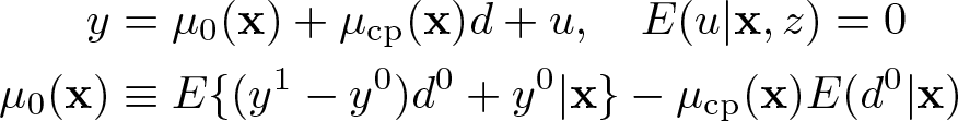
Note the “linear-in-d representation” for y in Lee (2021),

$\begin{array}{c}y={\mu }_0(x) +{\mu }_{cp}(x)d+u, E(u|x, z) = 0\\ {\mu }_0(x)\equiv E\{(y^1-y^0)d^0+y^0|x\}-{\mu }_{cp}(x)E(d^0|x)\end{array}$

which holds under d ⁰ ≤ d ¹ for any y as long as y ¹ − y ⁰ makes sense, where µ₀(x) is an unknown function of x and u is an error term. For exogenous d, set d = d ⁰ + (d ¹ − d ⁰)z equal to z to obtain (d ⁰ = 0, d ¹ = 1) (that is, everybody is a complier for exogenous d) and

${\mu }_{cp}(x) ={\mu }_1(x)\equiv E(y^1-y^0|x)\hspace{0.17em}and\hspace{0.17em}{\mu }_0(x) =E(y^0|x)$

The linear-in-d representation is a “causal reduced form (RF)” because it is an RF, not an structural form (that is, the data-generating model), which contains a causal parameter µ_cp(x) of interest. The causal RF holds for any form of µ_cp(x) and y.

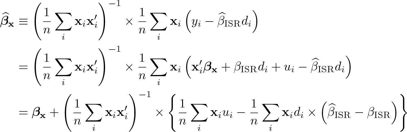
Rewrite the above linear-in-d representation as

$y-{\beta }_{ISR}d={\mu }_0(x) +\{{\mu }_{cp}(x)-{\beta }_{ISR}\}d+u$

Then the estimand of the OLS of y − β_ISR d on x is, with E^{− 1}(·) ≡ {E(·)} ^{− 1},

$\begin{array}{c}{E}^{-}{ }^1(xx\prime )E\{x(y-{\beta }_{ISR}d)\}=E^{-}{ }^1(xx\prime )E(x[{\mu }_0(x) +\{{\mu }_{cp}(x)-{\beta }_{ISR}\}d])\\ ={\beta }_x\hspace{0.17em}if\hspace{0.17em}{\mu }_0(x) =x\prime {\beta }_x\hspace{0.17em}and\hspace{0.17em}{\mu }_{cp}(x) ={\beta }_{ISR}\end{array}$

which is a sufficient condition for the slopes of x to be consistent for β _x . Note that under the sufficient condition, we have a linear model because

$y={\mu }_0(x) +{\mu }_{cp}(x)d+u=x\prime {\beta }_x+{\beta }_{ISR}d+u$

Denote the OLS of $y\hspace{0.17em}-\hspace{0.17em}{\widehat{\beta }}_{\text{ISR}}d$ on x as ${\widehat{\beta }}_X$ . Under the sufficient condition just mentioned, it holds that, with q in ${\widehat{\beta }}_{\text{ISR}}^q$ omitted,

$\begin{array}{l}{\widehat{\beta }}_x\equiv {\left(\frac{1}{n}{\displaystyle \sum _i{x}_i}{x^{\prime }}_i\right)}^{-1}\hspace{0.17em}\times \hspace{0.17em}\frac{1}{n}{\displaystyle \sum _i{x}_i}\left(y_i\hspace{0.17em}-\hspace{0.17em}{\widehat{\beta }}_{\text{ISR}}{d}_i\right)\\ \hspace{0.17em}=\hspace{0.17em}{\left(\frac{1}{n}{\displaystyle \sum _i{x}_i}{x^{\prime }}_i\right)}^{-1}\hspace{0.17em}\times \hspace{0.17em}\frac{1}{n}\hspace{0.17em}{\displaystyle \sum _i{x}_i}\left({x^{\prime }}_i{\beta }_x\hspace{0.17em}+\hspace{0.17em}{\beta }_{\text{ISR}}{d}_i\hspace{0.17em}+\hspace{0.17em}{u}_i\hspace{0.17em}-\hspace{0.17em}{\widehat{\beta }}_{\text{ISR}}{d}_i\right)\\ \hspace{0.17em}=\hspace{0.17em}{\beta }_x\hspace{0.17em}+\hspace{0.17em}{\left(\frac{1}{n}{\displaystyle \sum _i{x}_i}{x^{\prime }}_i\right)}^{-1}\hspace{0.17em}\times \hspace{0.17em}\left\{\frac{1}{n}\hspace{0.17em}{\displaystyle \sum _i{x}_i}{u}_i\hspace{0.17em}-\hspace{0.17em}\frac{1}{n}\hspace{0.17em}{\displaystyle \sum _i{x}_i}{d}_i\hspace{0.17em}\times \hspace{0.17em}\left({\widehat{\beta }}_{\text{ISR}}\hspace{0.17em}-\hspace{0.17em}{\beta }_{\text{ISR}}\right)\right\}\end{array}$

Be aware that ${\widehat{\beta }}_x$ here is not the same as the x-slope in the OLS of y on (x , d), because the slope estimator of d in this OLS is not ${\widehat{\beta }}_{\text{ISR}}$ .

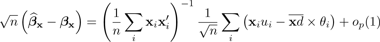
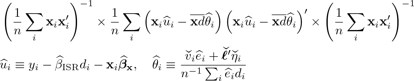
Let the influence function of ${\widehat{\beta }}_{\text{ISR}}$ be θ_i : $\sqrt{n}\left({\widehat{\beta }}_{\text{ISR}}\hspace{0.17em}-\hspace{0.17em}{\beta }_{\text{ISR}}\right)\hspace{0.17em}=\hspace{0.17em}{n}^{-1/2}{\displaystyle {\sum }_i{\theta }_i}+\hspace{0.17em}{o}_p\hspace{0.17em}(1)$ ; the form of θ_i is shown shortly. Then, using the preceding display, we obtain

$\sqrt{n}\left({\widehat{\beta }}_x\hspace{0.17em}-\hspace{0.17em}{\beta }_x\right)\hspace{0.17em}=\hspace{0.17em}{\left(\frac{1}{n}\hspace{0.17em}{\displaystyle \sum _i{x}_i}{x^{\prime }}_i\right)}^{-1}\hspace{0.17em}\frac{1}{\sqrt{n}}\hspace{0.17em}{\displaystyle \sum _i\left(x_i{u}_i\hspace{0.17em}-\hspace{0.17em}\overline{xd}\hspace{0.17em}\times \hspace{0.17em}{\theta }_i\right)\hspace{0.17em}}+\hspace{0.17em}{o}_p(1)$

where $\overline{xd}\equiv n^{-1}\hspace{0.17em}{\displaystyle {\sum }_i{x}_i{d}_i}$ . Hence, $\sqrt{n}\left({\widehat{\beta }}_x-{\beta }_x\right)$ is asymptotically normal with the variance estimated with

$\begin{array}{l}{\left(\frac{1}{n}{\displaystyle \sum _i{x}_i}{x}_i^{\prime }\right)}^{-1}\times \hspace{0.17em}\frac{1}{n}{\displaystyle \sum _i\left(x_i{\widehat{u}}_i-\overline{xd}{\widehat{\theta }}_i\right)}\hspace{0.17em}{\left(x_i{\widehat{u}}_i-\overline{xd}{\widehat{\theta }}_i\right)}^{\prime }\hspace{0.17em}\times \hspace{0.17em}{\left(\frac{1}{n}{\displaystyle \sum _i{x}_i}{x}_i^{\prime }\right)}^{-1}\hfill \\ {\widehat{u}}_i\equiv \hspace{0.17em}{y}_i-\hspace{0.17em}{\widehat{\beta }}_{\text{ISR}}{d}_i-x_i{\widehat{\beta }}_x,\hspace{1em}{\widehat{\theta }}_i\hspace{0.17em}\equiv \hspace{0.17em}\frac{{\stackrel{⌣}{v}}_i{\widehat{e}}_i+{\stackrel{⌣}{\mathcal{l}}}^{\prime }{\stackrel{⌣}{\eta }}_i}{n^{-1}\hspace{0.17em}{\displaystyle {\sum }_i{\widehat{e}}_i{d}_i}}\hfill \end{array}$

Bear in mind that ${\widehat{\beta }}_x$ is not of primary interest. Rather, ${\widehat{\beta }}_x$ and its asymptotic distribution derived under the restrictive conditions [µ₀(x) = x′β_x and µ_cp(x) = β_ISR] are just to give some idea on the contribution of x to µ₀(x) because having only one estimate ${\widehat{\beta }}_{\text{ISR}}$ at the end of data analysis may leave the researcher feeling somewhat “unfulfilled”.

3 The psr command

The command psr implements OLS with a PSR and an IVE with an ISR.

3.1 Syntax

The syntax for OLS with a PSR is

psr depvar treatment_var covariates [if] [in ][, logit order( # ) useprob auxiliary verbose vverbose ]

when the binary treatment variable is exogenous. The syntax for an IVE with ISRs is

psr depvar ( treatment_var = instrument ) covariates [if] [in ] [, logit order( # ) useprob auxiliary verbose vverbose ]

when the endogenous binary treatment variable is instrumented by an exogenous binary instrument. The covariates should be exogenous always.

3.2 Options

logit specifies to use logit instead of probit for propensity or IS regression.

order( # ) specifies the maximum polynomial order q for predicting the dependent variable by the fitted linear index or the fitted probability. The default is order(2).

useprob uses the fitted probability for the prediction of the dependent variable instead of the fitted linear index. By default, the linear index is used.

auxiliary reports results from auxiliary regression for covariate slopes with the standard errors.

verbose displays all intermediate step results.

vverbose is the same as the auxiliary and verbose options used together.

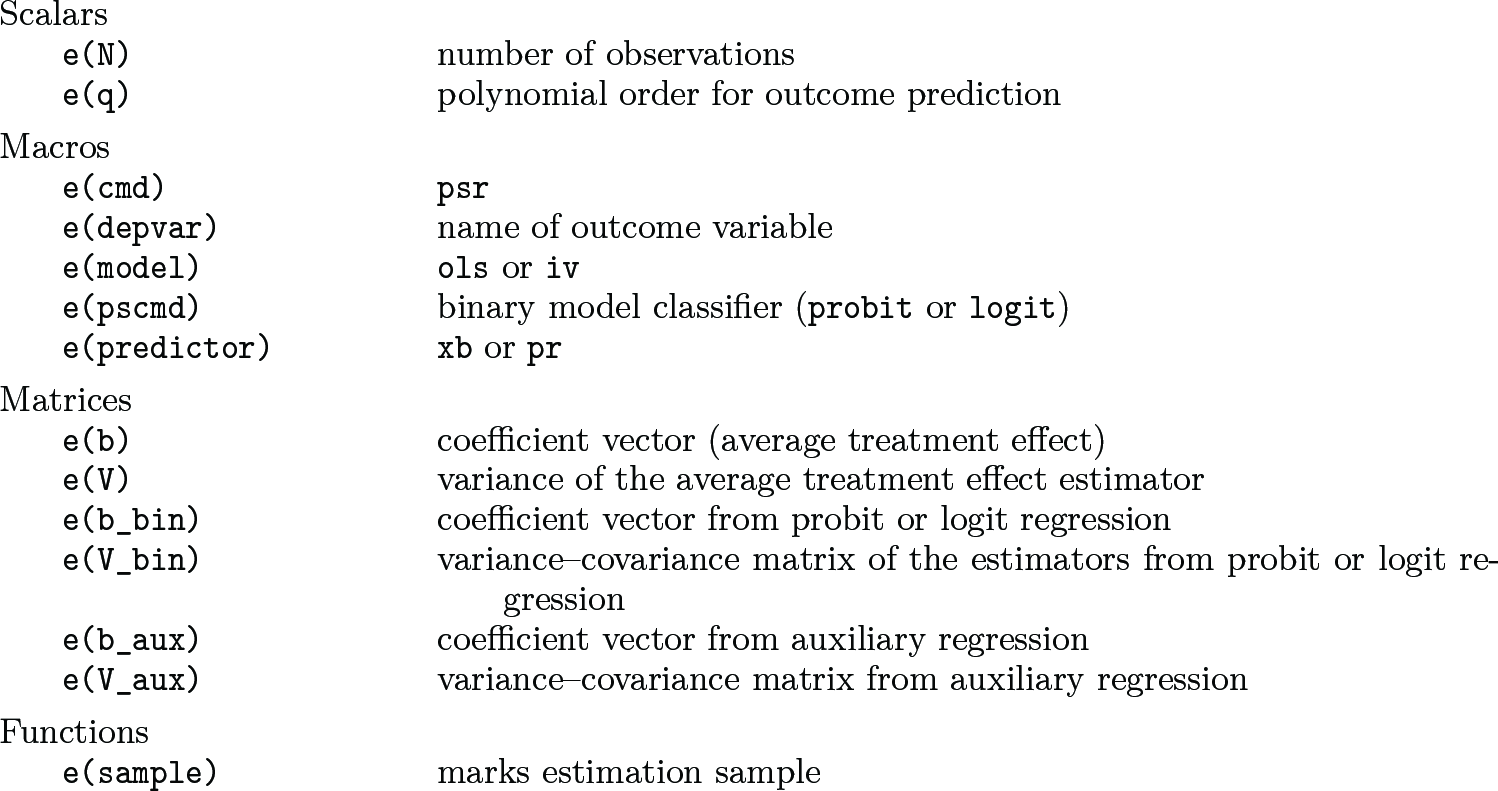
3.3 Stored results

psr stores the following in e():

4 Applications

We present two applications in this section: flu vaccine effect on hospitalization or not (Lee 2021; Ding and Lu 2017) and education effect on wage (Lee 2021).

4.1 Flu vaccine effect on hospitalization

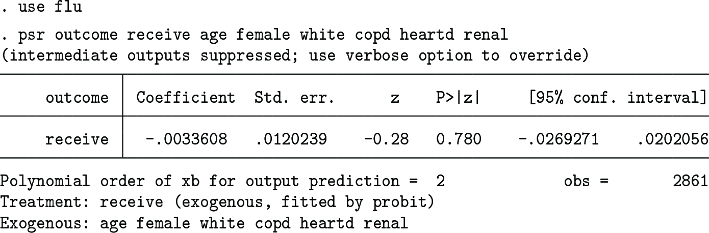
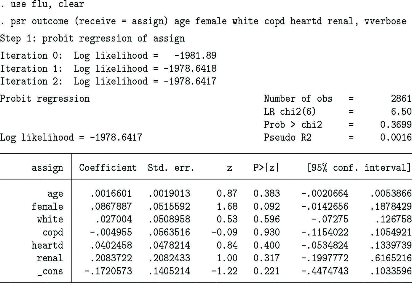
The first application is flu vaccine effect on hospitalization or not. flu.dta is prepared using the Ding and Lu (2017) data. The outcome variable is outcome, the treatment variable is receive, and the exogenous covariates are age, female, white, copd, heartd, and renal. Lee (2021) allows the treatment to be endogenous and instruments it with assign. We consider exogenous and endogenous treatments for the sake of illustration.

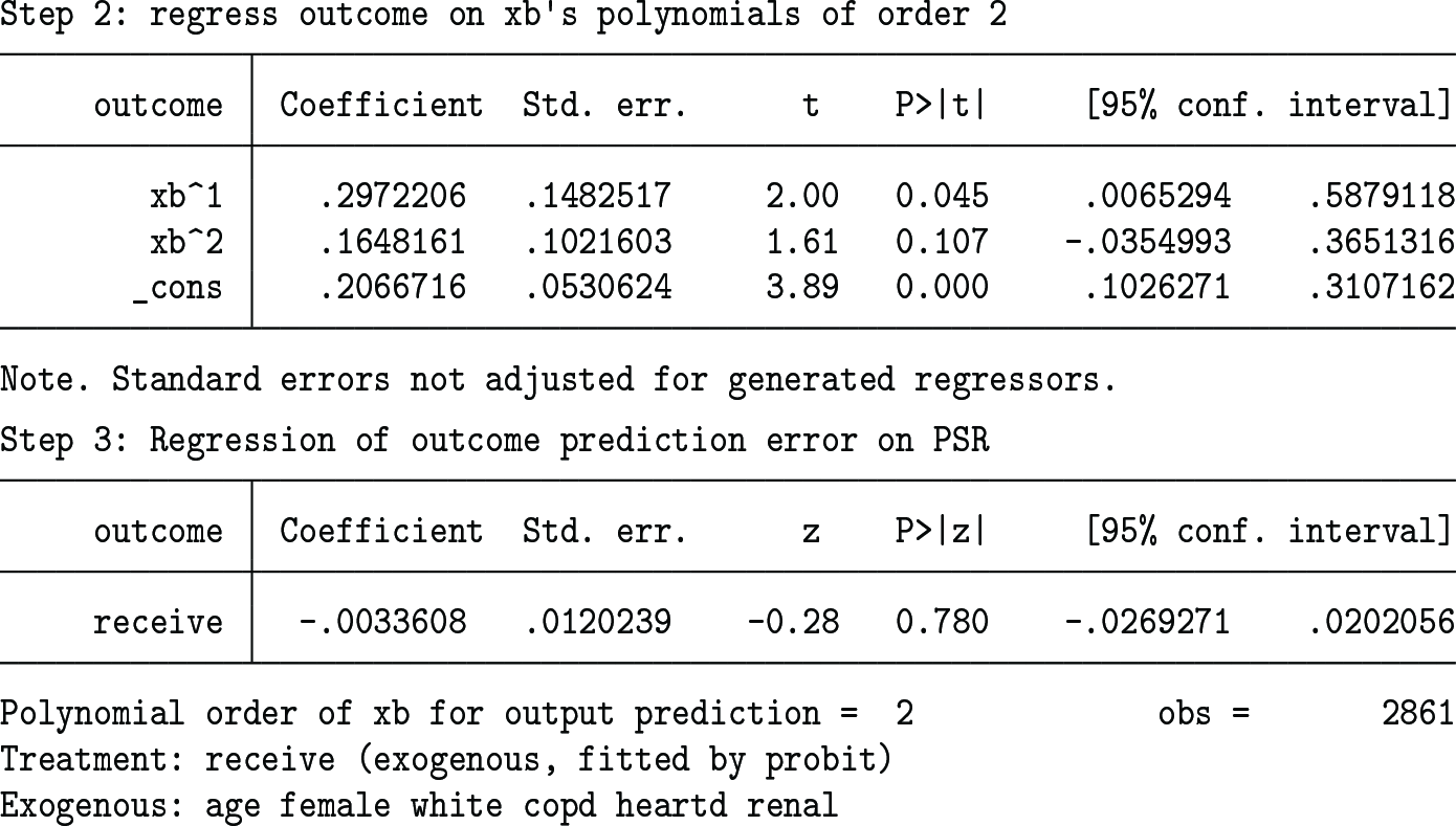
With the treatment assumed to be exogenous, the psr command invoked with the default options gives the following results, where the OW average treatment effect is small in magnitude and is statistically insignificant:

In this OLS result, the treatment effect (−0.0033608) is obtained as follows: The treatment variable (receive) is regressed on the covariates (age, female, white, copd, heartd, and renal) by probit, and the outcome prediction error is obtained by regressing the outcome variable (outcome) on the linear index (xb) and its square. The OW average treatment effect is then obtained by the OLS regression of the outcome prediction error on the PSR.

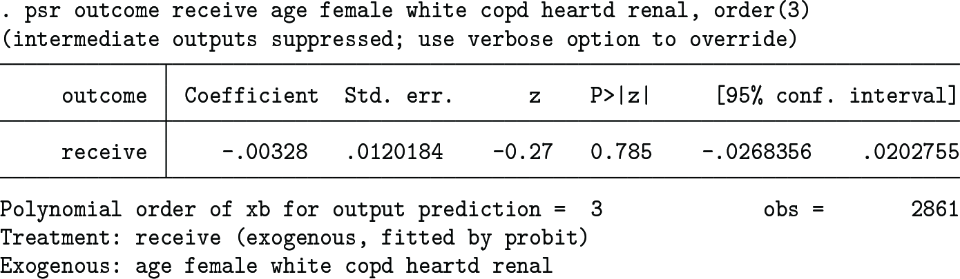
A third-order polynomial of the linear index can be added to the outcome prediction regression, which yields the following result:

The results change only marginally.

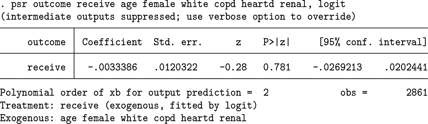
Logit can replace probit by using the logit option, as the following example illustrates:

The results are almost identical to those by the probit regression.

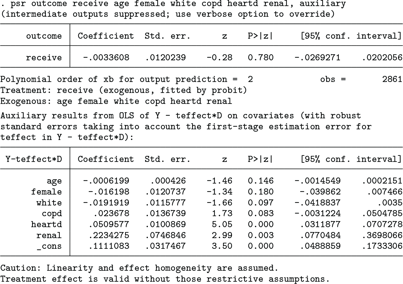
The auxiliary covariate slopes (derived under restrictive conditions in section 2.4 to make the y model linear) are reported as follows when the auxiliary option is used:

The results from the auxiliary regression of $y-\widehat{\beta }d$ on the covariates are displayed after the estimated OW treatment effect. The reported standard errors are corrected for the first-stage estimation error, and cautionary warnings are noted.

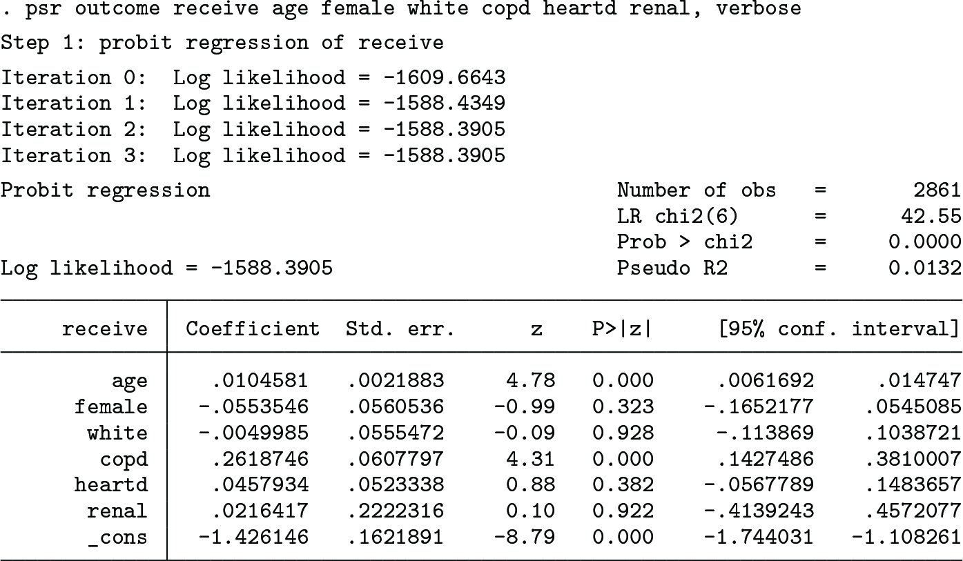
All the intermediate-step results are displayed if the verbose option is used:

The displayed results are self-evident. The vverbose option is identical to verbose and auxiliary used together.

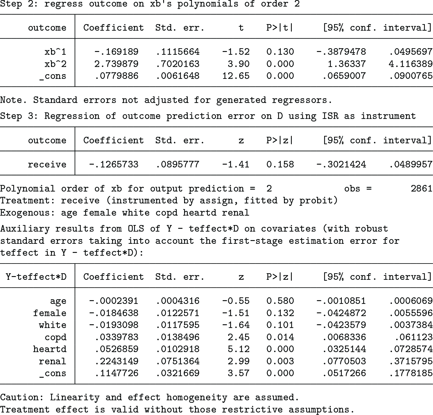
We have so far assumed that the treatment (receive) is exogenous. When it is possibly endogenous and is instrumented by assign, the results (using the vverbose option to display all intermediate steps and the auxiliary covariate slopes) are as follows:

First, the instrument (assign) is regressed on the covariates. Second, the outcome variable (outcome) is fit using the polynomials of the linear index up to the second order. Finally, the outcome prediction error is regressed on the treatment variable (receive) using the ISR as the instrument. The estimated OW average treatment effect is −0.1265733, which is much larger than the one obtained under the treatment exogeneity assumption, though it is still statistically insignificant at the 10% level (p-value = 0.158). Lee (2021, 626) shows that the usual linear-model IVE yields almost the same effect estimate, −0.13, with or without x controlled for. The estimated covariate slopes are presented as the final output.

4.2 Education effect on wage

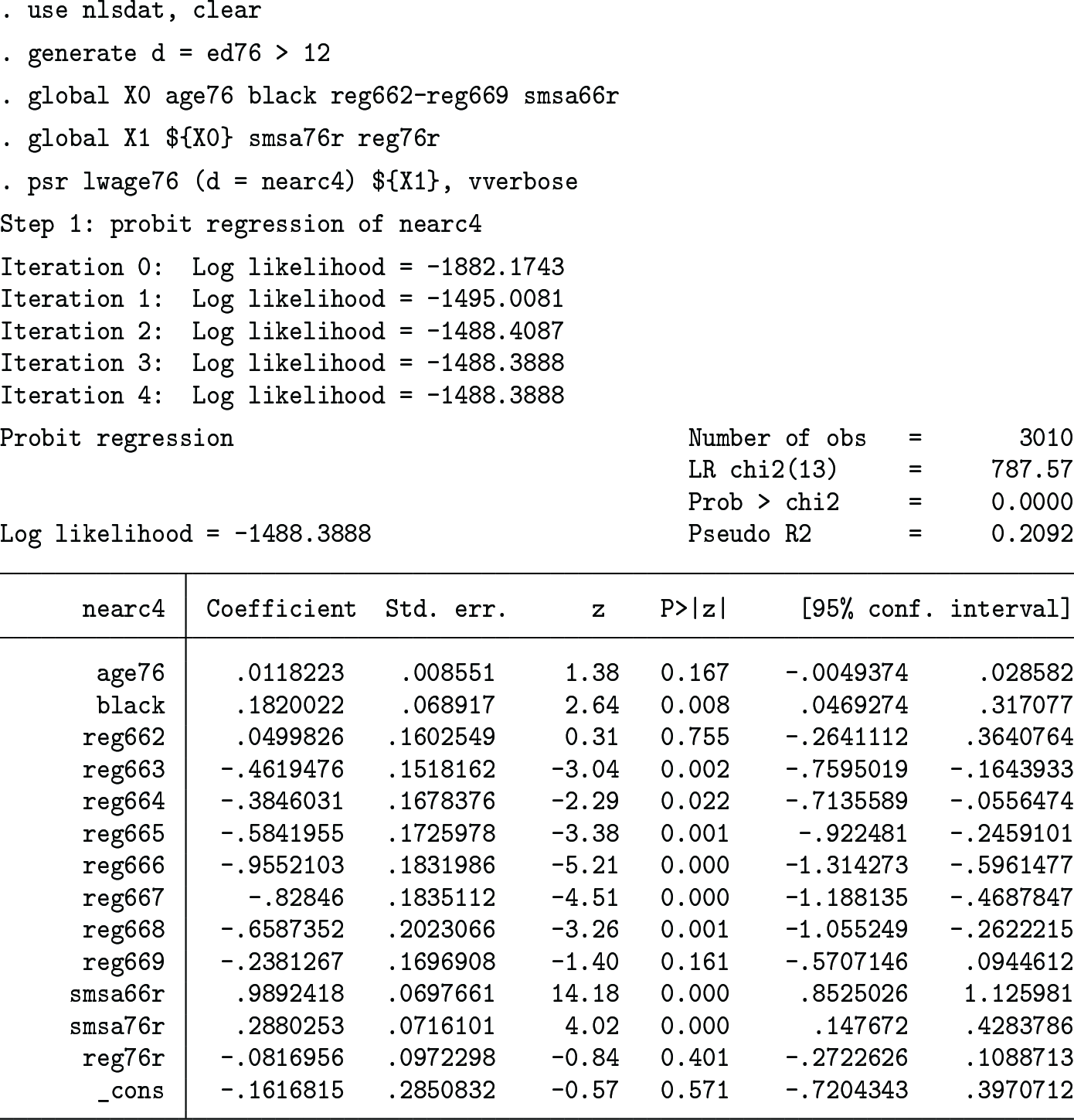
Our second empirical analysis is for education effect on wage (Lee 2021) based on Card (1995). nlsdat.dta is prepared using files at https://davidcard.berkeley.edu/data_sets.html. The variable names to appear below are taken from the codebook provided in this URL.

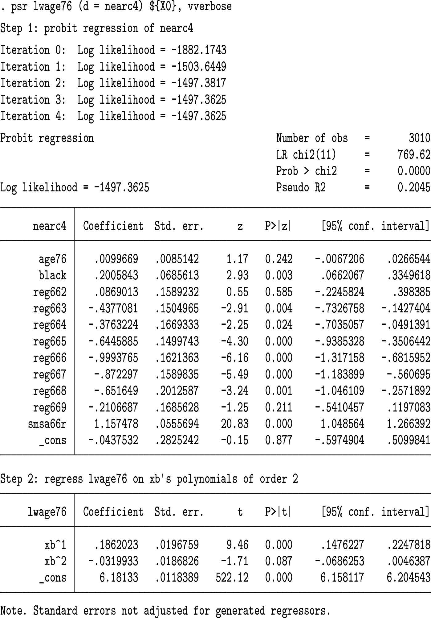
The outcome variable is ln(wage) in 1976 (lwage76), the treatment variable (d) is the binary indicator for the schooling years in 1976 (ed76) to exceed 12, the instrument (z) is for whether one grew up near a four-year college (nearc4), and the covariates (x) consist of 1, age (age76), dummy for black (black), dummies for nine residence regions in 1966 (reg662–reg669, with reg661 as the base category), dummy for living in a standard metropolitan statistical area in 1966 (smsa66r), dummy for living in a standard metropolitan statistical area in 1976 (smsa76r), and dummy for living in the South in 1976 (reg76r).

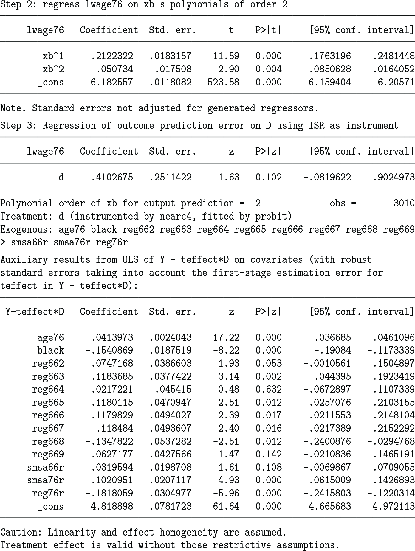
Lee (2021) presented two results with and without smsa76r and reg76r because of the possibility of them being affected by d. With smsa76r and reg76r included, the IVE regression of the outcome prediction error on the treatment using the instrument propensity residual as the instrument gives the following results (with the vverbose option used to show all the intermediate-step results and the auxiliary covariate slopes):

The OW average treatment effect is estimated to be 0.4102675 (with the robust standard error 0.2511422), as is shown in the Step 3 part of the output. Lee (2021, 628) shows that the usual linear-model IVE with x controlled yields the effect estimate 0.43 (with the robust standard error 0.24), which differs little from the OW average treatment effect result.

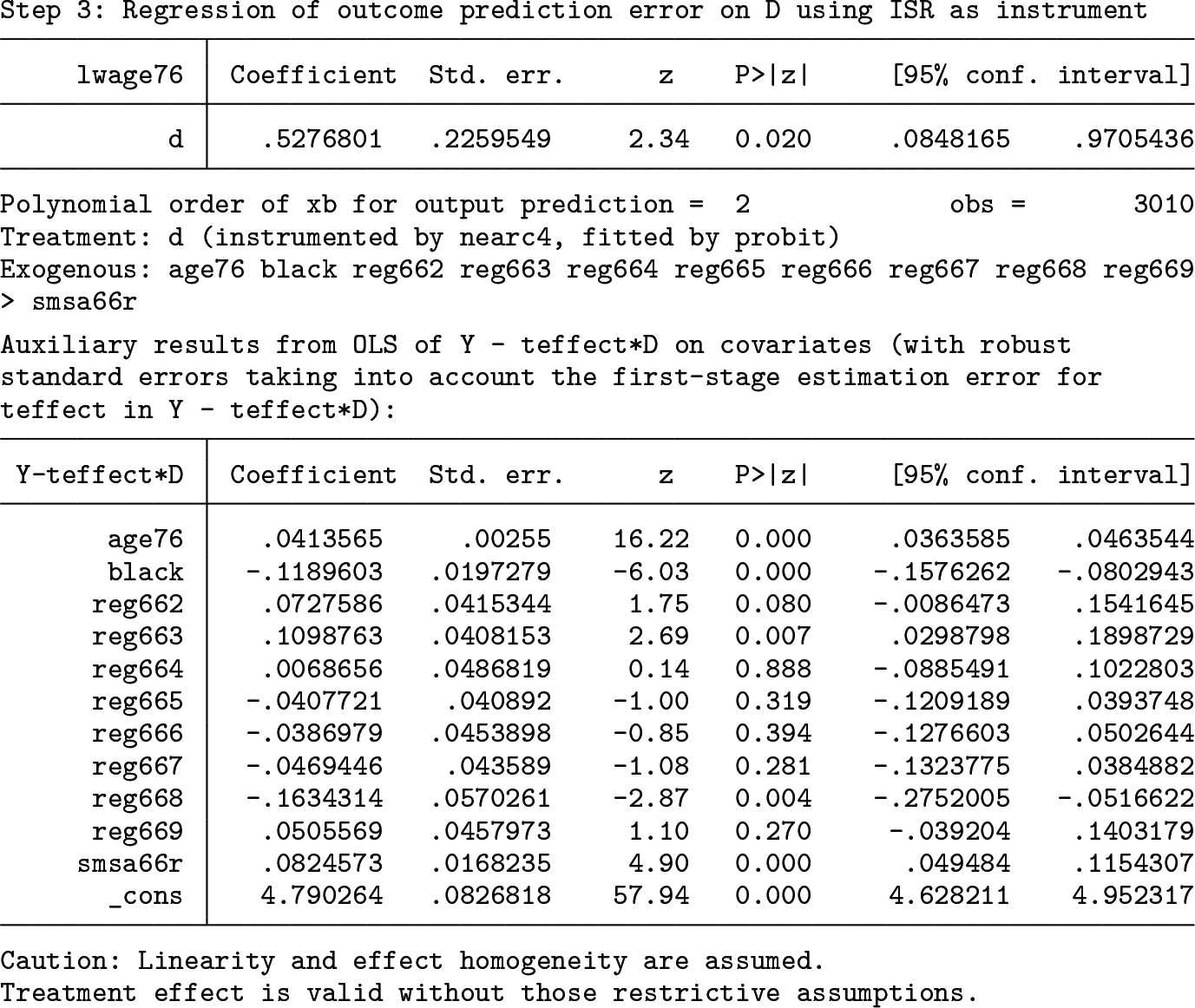
With smsa76r and reg76r excluded from the covariate list, the results change to the following:

The estimated OW average treatment effect is 0.5276801 (with the robust standard error 0.2259549), which is statistically significant at the 5% level (p-value = 0.020). Lee (2021, 628) shows that the usual linear-model IVE with x controlled yields the effect estimate 0.55 (with the robust standard error 0.22), which differs little from the OW average treatment effect result.

5 Conclusions

In finding the effect of a binary treatment d, practitioners often apply OLS to LDVs y, despite the fact that the linear model is untenable. Also, COVID-19 recently demonstrated how heterogeneous treatment effects can be, yet linear models typically assume a constant effect. This brought up an important question: What does the OLS estimate when the effect is x-heterogeneous, being a function µ₁(x) of x, and the linear model is invalid?

The answer in the literature is that the effect estimated by the OLS is a weighted average E{ω(x)µ₁(x)}, where the weight ω(x) is high for those with their PS π _x ≡ E(d| x) ≃0.5 and low for those with π _x ≃ 0, 1; ω(x) is called the OW. However, this answer requires that π _x be equal to the linear projection of d on x, which unfortunately rarely holds in reality. Without this condition, the OLS can be consistent for a nonzero number even when µ₁(x) = 0. This brought up another question: Can E{ω(x)µ₁(x)} be estimated without the restrictive condition?

To this question, Lee (2018) showed that the OLS of y on d − π _x (“OLS_PSR”) is consistent for E{ω(x)µ₁(x)} without the restrictive condition. Going further, Lee (2021) showed that when d is endogenous with a binary instrument z, the IVE of y on d with instrument z − ζ _x (“IVE_ISR”), where ζ _x ≡ E(z| x) is the instrument score (IS), is consistent for a modified OW average of µ₁(x). This article reviewed OLS_PSR and IVE_ISR and then provided the command psr to implement OLS_PSR and IVE_ISR, which are applicable to any µ₁(x) and any y (continuous, count, binary, etc.).

Because both OLS_PSR and IVE_ISR are implemented by specifying π _x and ζ _x as probit (or logit), one concern in OLS_PSR and IVE_ISR is misspecifications in the probit or logit for π _x or ζ _x . To make OLS_PSR and IVE_ISR robust to such misspecifications, the actually implemented version of OLS_PSR and IVE_ISR uses, respectively, y − E(y|π _x ) and y − E(y|ζ _x ) instead of y. This idea is closely related to the recent “double debiasing” idea for robustness to misspecifications in nuisance functions such as π _x or ζ _x , where y − E(y| x) is used instead of y and then a machine-learning method estimates E(y| x).

In our two empirical illustrations where one outcome is binary and the other is continuous, OLS_PSR and IVE_ISR yielded estimates very close to those of the usual linearmodel OLS and IVE. This demonstrates that OLS_PSR and IVE_ISR reduce to the usual linear-model OLS and IVE when π _x is the same as the linear projection; otherwise, OLS_PSR and IVE_ISR would still provide the OW average treatment effect. By providing the command, we hope that OLS_PSR and IVE_ISR are more widely applied because they require neither any linear approximation argument nor constant effect assumption.

As far as we can see, there are two remaining issues in OLS_PSR and IVE_ISR; one is easy to address, but the other is not. The first issue is the robustness to misspecifications in π _x and ζ _x because it is not “full” yet. If the x-centered variables {y − E(y| x), d − π _x , z − ζ _x } are used in the OLS_PSR and IVE_ISR, then OLS_PSR and IVE_ISR will be fully double debiasing. This will be done in the near future, and a command will become available before long because the research is underway. The other issue is the OW: If one objects to OW, are there any other sensible weighting schemes to adopt? The answer would be yes, but it is unlikely that any sensible weighting scheme other than OW is compatible with OLS- and IVE-based approaches.

7 Programs and supplemental material

Supplemental Material, sj-zip-1-stj-10.1177_1536867X241233645 - Ordinary least squares and instrumental-variables estimators for any outcome and heterogeneity

Supplemental Material, sj-zip-1-stj-10.1177_1536867X241233645 for Ordinary least squares and instrumental-variables estimators for any outcome and heterogeneity by Myoung-jae Lee and Chirok Han in The Stata Journal