pystacked: Stacking generalization and machine learning in Stata

Abstract

The pystacked command implements stacked generalization (Wolpert, 1992, Neural Networks 5: 241–259) for regression and binary classification via Python’s scikit-learn. Stacking combines multiple supervised machine learners—the “base” or “level-0” learners—into one learner. The currently supported base learners include regularized regression, random forest, gradient boosted trees, support vector machines, and feed-forward neural nets (multilayer perceptron). pystacked can also be used as a “regular” machine learning program to fit one base learner and thus provides an easy-to-use application programming interface for scikit-learn‘s machine learning algorithms.

1 Introduction

When faced with a new prediction or classification task, it is rarely obvious which machine learning algorithm is best suited. A common approach is to evaluate the performance of a set of machine learners on a holdout partition of the data or via crossvalidation and then select the machine learner that minimizes a chosen loss metric. However, this approach is incomplete because combining multiple learners into one final prediction might lead to superior performance compared with each individual learner. This possibility motivates stacked generalization, or simply “stacking” (see Wolpert [1992] and Breiman [1996]). Stacking is a form of model averaging. Theoretical results in van der Laan, Polley, and Hubbard (2007) support the use of stacking because it performs asymptotically at least as well as the best-performing individual learner as long as the number of base learners is not too large.

In this article, we introduce pystacked, a command for stacking regression and binary classification in Stata. pystacked allows users to fit multiple machine learning algorithms via Python’s scikit-learn (Pedregosa et al. 2011; Buitinck et al. 2013) and combine these into one final prediction as a weighted average of individual predictions. pystacked adds to the growing number of programs for machine learning in Stata, including lassopack for regularized regression (Ahrens, Hansen, and Schaffer 2020), rforest for random forests (Schonlau and Zou 2020), and svm for support vector machines (Guenther and Schonlau 2016, 2018). Similarly to pystacked, Cerulli (2022) and Droste (2022) provide an interface to scikit-learn in Stata. mlrtime allows Stata users to make use of R’s parsnip machine learning library (Huntington-Klein 2021). pystacked differs from these in that it is, to our knowledge, the first to make stacking available to Stata users. Furthermore, pystacked can also be used to fit one machine learner and thus provides an easy-to-use and versatile application programming interface to scikit-learn’s machine learning algorithms.

Stacking is widely used in applied predictive modeling in many disciplines—for example, predicting mortality (Hwangbo et al. 2022), bankruptcy filings (Liang et al. 2020; Fedorova et al. 2022), or temperatures (Hooker, Duveiller, and Cescatti 2018). However, the use of stacking as a method and pystacked as a program is not restricted only to pure prediction or classification tasks. A growing literature exploits machine learning to facilitate causal inference (for an overview, see Athey and Imbens [2019]). Indeed, a motivation for writing pystacked is that it can be used in combination with ddml (Ahrens et al. Forthcoming, 2023), which implements the double-debiased machine learning (DDML) methodology of Chernozhukov et al. (2018). DDML uses cross-fitting, a form of iterative sample splitting, which allows leveraging of a wide class of supervised machine learners, including stacking, for the estimation of causal parameters. For instance, in the context of DDML, stacking can be used to estimate the conditional expectation of an outcome with respect to confounders or propensity scores.

We stress that pystacked relies on Python’s scikit-learn (version 0.24 or higher) and the ongoing work of the scikit-learn contributors. Thus, pystacked relies on Stata’s Python integration, which was introduced in Stata 16.0. We kindly ask users to cite scikit-learn along with this article when using pystacked. Throughout, we refer to version 0.7.1 of pystacked, which is the latest version at the time of writing. Please check for updates to pystacked regularly, and consult the help file to be informed about new features. The pystacked help file includes information on how to install a recent Python version and set up Stata’s Python integration.

Section 2 introduces stacking. Section 3 presents the main features of the pystacked program. Section 4 demonstrates the use of the program using examples.

2 Methodology

In this section, we briefly summarize the stacking approach for regression and binary classification tasks. Van der Laan and Rose (2011) provides a book-length treatment; for a concise textbook treatment, see Hastie, Tibshirani, and Friedman (2009).

We first focus on stacking for regression problems where the aim is to predict the continuous outcome y_i using predictors x _i . The idea of stacking is to combine a set of “base” (or “level-0”) learners using a “final” (or “level-1”) estimator. It is advisable to include a relatively large and diverse set of base learners to capture different types of patterns in the data. The same algorithm can also be included more than once using different tuning or hypertuning parameters. Typical choices for base learners are regularized regression or ensemble methods, such as random forests or gradient boosting.

In the first step of stacking, we obtain cross-validated predicted values ${\widehat{y}}_{\left(j\right),\hspace{0.17em}i\hspace{0.17em}}^{-k\hspace{0.17em}\left(i\right)}$ for each base learner j and observation i. The superscript −k(i) indicates that we form the cross-validated predicted value for observation i by fitting the learner to all folds except fold k(i), which is the fold that includes observation i. The use of cross-validation is necessary because stacking would otherwise give more weight to base learners that suffer from overfitting. The second step is to fit a final learner using the observed y_i as the outcome and the cross-validated predicted values ${\widehat{y}}_{\left(1\right),\hspace{0.17em}i\hspace{0.17em}}^{-k\hspace{0.17em}\left(i\right)}$ ,…, ${\widehat{y}}_{\left(J\right),\hspace{0.17em}i\hspace{0.17em}}^{-k\hspace{0.17em}\left(i\right)}$ as predictors. A typical choice for the final learner is constrained least squares, which enforces the stacking weights to be nonnegative and sum to one. This restriction facilitates the interpretation of stacking as a weighted average of base learners and may lead to better performance (Breiman 1996; Hastie, Tibshirani, and Friedman 2009). Algorithm 1 summarizes the stacking algorithm for regression problems as it is implemented in pystacked.

Algorithm 1: Stacking regression

Cross-validation:

Split the sample I = {1,…, n} randomly into K partitions of approximately equal size. These partitions are referred to as “folds”. Denote the set of observations in fold k = 1,…, K as I_k and its complement as $I_k^c$ such that $I_k^c\hspace{0.17em}=\hspace{0.17em}I\backslash I_k$ . I_k constitutes the step-k validation set and $I_k^c$ the step-k training sample.

For each fold k = 1,…, K and each base learner j = 1,…, J, fit the supervised machine learner j to the training data $I_k^c$ and obtain out-of-sample predicted values ${\widehat{y}}_{\left(j\right),\hspace{0.17em}i\hspace{0.17em}}^{-k}$ for i ∊ I_k .

Final learner: Fit the final learner to the full sample. The default choice is nonnegative least squares with the additional constraint that coefficients sum to one:

$\underset{w_1,\dots ,w_J}{\min }\hspace{0.17em}{{\displaystyle \sum _{i=1}^n\hspace{0.17em}\left(y_i\hspace{0.17em}-\hspace{0.17em}{\displaystyle \sum _{j=1}^J\hspace{0.17em}{w}_j{\widehat{y}}_{\left(j\right),\hspace{0.17em}i\hspace{0.17em}}^{-k\hspace{0.17em}\left(i\right)}}\right)}}^2 \hspace{0.17em}\text{s.t. }\hspace{1em}{w}_j\hspace{0.17em}\ge \hspace{0.17em}0,\hspace{1em}{\displaystyle \sum _{j=1}^J\hspace{0.17em}{w}_j}\hspace{0.17em}=\hspace{0.17em}1$

The stacking predicted values are defined as ${\widehat{y}}_i^{\star }\hspace{0.17em}=\hspace{0.17em}{\displaystyle {\sum }_j\hspace{0.17em}{\widehat{w}}_j{\widehat{y}}_{(j),\hspace{0.17em}i}}$ where ${\widehat{w}}_j$ is the estimated stacking weight corresponding to learner j and ${\widehat{y}}_{(j),\hspace{0.17em}i}$ are the predicted values from refitting learner j on the full sample I.

It is instructive to compare step 2 with the classical “winner-takes-all” approach that selects one base learner as the one that exhibits the lowest cross-validated loss. Stacking, in contrast, may assign nonzero weights to multiple base learners, thus combining their strengths to produce an overall predictor that can be better than any of the individual base learners. Other choices for the final learner are possible. In addition to the default final learner, pystacked supports, among others, nonnegative least squares without the constraint ∑ w_j = 1, ridge regression, the aforementioned “winner-takes-all” approach that selects the base learner with the smallest cross-validated mean squared error, and unconstrained least squares.

2.1 Stacking classification

Stacking can be applied similarly to classification problems. pystacked supports stacking for binary classification problems where the outcome y_i takes the values 0 or 1. The main difference from stacking regression is that ${\widehat{y}}_{\left(j\right),\hspace{0.17em}i\hspace{0.17em}}^{-k}$ represents cross-validated predicted probabilities.

2.2 Base learners

In the next paragraphs, we briefly describe the base learners supported by pystacked and highlight central tuning parameters. We repeat that each of the machine learners discussed below can be fit using pystacked as a regular stand-alone machine learner without the stacking layer.

Note that it is beyond the scope of the article to describe each learner in detail. Familiarity with linear regression, logistic regression, and classification and regression trees is assumed. We recommend consulting machine learning textbooks, for example, Hastie, Tibshirani, and Friedman (2009), for more detailed discussion.

Regularized regression imposes a penalty on the size of coefficients to control overfitting. The lasso penalizes the absolute size of coefficients, whereas the ridge penalizes the sum of squared coefficients. Both methods shrink coefficients toward zero, but only the lasso yields sparse solutions where some coefficient estimates are set to exactly zero. The elastic net combines lasso- and ridge-type penalties. For classification tasks with a binary outcome, logistic versions of lasso, ridge, and elastic net are available.

The severity of the penalty is most commonly chosen by cross-validation. For lasso only, pystacked also supports selecting the penalty by the Akaike information criterion (AIC) or Bayesian information criterion (BIC). The use of AIC or BIC has the advantage that it is computationally less intensive than cross-validation. Ahrens, Hansen, and Schaffer (2020) compare the two approaches.

Random forests rely on fitting many regression or decision trees on bootstrap samples of the data. The random forest prediction is obtained as the average across individual trees. A crucial aspect of random forests is that, at each split when growing a tree, one may consider only a random subset of predictors. This restriction aims at decorrelating the individual trees. Central tuning parameters are the number of trees ( n_estimators()), the maximum depth of individual trees ( max_depth()), the minimum number of observations per leaf ( min_samples_leaf()), the number of features to be considered at each split ( max_features()), and the size of the bootstrap samples ( max_samples()).

Gradient boosted trees also rely on fitting many trees. In contrast to random forests, these trees are fit sequentially to the residuals from the current model. The learning rate determines how much the latest tree contributes to the overall model. Individual trees are usually fit to the whole sample, although subsampling is possible. In addition to tuning parameters relating to the trees, the learning rate ( learnings_rate()) and the number of trees ( n_estimators()) are the most important tuning parameters.

Support vector machines. Support vector classifiers span a hyperplane that separates observations by their outcome class. The hyperplane is chosen to maximize the distance ( margin) to correctly classified observations while allowing for some classification errors. The tuning parameter C ( C()) controls the frequency and degree of classification mistakes. The hyperplane can be either linear or fit using kernels. The support vector machine algorithm can also be adapted for regression tasks. To this end, the hyperplane is constructed to include as many observations as possible in a tube of size 2ϵ around the hyperplane. Central tuning parameters for regression are ϵ ( epsilon()) and C ( C()), which determine the cost of observations outside of the tube.

Feed-forward neural networks consist of hidden layers that link the predictors (referred to as “input layers”) to the outcome. Each hidden layer is composed of multiple units (nodes) that pass signals to the next layer using an activation function. Central tuning parameters are the choice of the activation function ( activation()) and the number and size of hidden layers ( hidden_layer_sizes()). Further tuning choices relate to stochastic gradient descent algorithms, which are typically used to fit neural networks. The default solver is Adam (Kingma and Ba 2017). The option early_stopping can be used to set aside a random fraction of the data for validation. The optimization algorithm stops if there is no improvement in performance over a prespecified number of iterations (see related options n_iter_no_change() and tol()).

3 Program

This section introduces the program pystacked and its main features. pystacked offers two alternative syntaxes to the user (see sections 3.1 and 3.2). The two syntaxes offer the same functionality and are included to accommodate different user preferences. Sections 3.3 and 3.4 list postestimation commands and general options, respectively. Section 3.5 discusses supported base learners. Section 3.6 is a note on learner-specific predictors. Section 3.7 explains the pipeline feature.

3.1 Syntax 1

The first syntax uses methods() to select base learners, where string is a list of base learners. Options are passed on to base learners via cmdopt1(), cmdopt2(), etc. That is, base learners can be specified, and options are passed on in the order in which they appear in methods() (see section 3.5). Likewise, the pipe∗ () option can be used for preprocessing predictors within Python on the fly, where ∗ is a placeholder for 1, 2, etc. (see section 3.7). Finally, xvars∗ () allows the specification of a learner-specific variable list of predictors.

pystacked depvar predictors [if] [in] [ , methods( string ) cmdopt1( string )

[ cmdopt2( string ) [… ]] pipe1( string ) [ pipe2( string ) [… ]]

xvars1( predictors ) [ xvars2( predictors ) [… ]] general_options]

general_options are discussed in section 3.4 below.

3.2 Syntax 2

In the second syntax, base learners are added before the comma using method(), along with further learner-specific settings, and separated by ||.

pystacked depvar [indepvars] || method( string ) options( string )

pipeline( string ) xvars( predictors ) [ || method( string ) options( string )

pipeline( string ) xvars( predictors ) || … ||] [if] [in] [ , general_options]

3.3 Postestimation commands

Predicted values

To get predicted values:

predict type newname [if] [in] [, xb pr]

To get fitted values for each base learner:

predict type stub [if] [in] [ , basexb cvalid]

Predicted values (in and out of sample) are calculated when pystacked is run and stored in Python memory. predict pulls the predicted values from Python memory and saves them in Stata memory. This storage structure means that no changes on the data in Stata memory should be made between the pystacked call and the predict call. If changes to the dataset are made, predict will return an error.

The option basexb returns predicted values for each base learner. By default, the predicted values from refitting base learners on the full estimation sample are returned. If combined with cvalid, the cross-fitted predicted values are returned for each base learner.

Tables

After estimation, pystacked can report a table of in-sample (both cross-validated and full-sample) and, optionally, out-of-sample (or holdout sample) performances for both the stacking regression and the base learners. For regression problems, the table reports the root mean squared prediction error (RMSPE). For classification problems, a confusion matrix is reported. The default holdout sample used for out-of-sample performance with the holdout option is all observations not included in the estimation. Alternatively, the user can specify the holdout sample explicitly using holdout(). The table can be requested after estimation as a replay command or as part of the pystacked estimation.

pystacked [ , table [ ( options )] holdout [ ( varname )]]

Graphs

pystacked can also create graphs of in-sample and, optionally, out-of-sample performance for both the stacking regression and the base learners. For regression problems, the graphs compare predicted and actual values of depvar. For classification problems, the default is to generate receiver operator characteristic (ROC) curves. Optionally, histograms of predicted probabilities are reported. As with the table option, the default holdout sample used for out-of-sample performance is all observations not included in the estimation, but the user can instead specify the holdout sample explicitly. The table can be requested after estimation or as part of the pystacked estimation command. The graph option on its own reports the graphs using pystacked‘s default settings. Because graphs are produced using Stata’s twoway, roctab, and histogram commands, the user can control either the combined graph ( graph()) or the individual learner graphs ( lgraph()) by passing options to these commands.

pystacked [ , graph [ ( options )] lgraph [ ( options )] histogram

holdout [ ( varname )]]

3.4 General options

A full list of general options is provided in the pystacked help file. We list only the most important general options here:

type( string )allows regress for regression problems or classify for classification problems. The default is regression.

finalest( string ) selects the final estimator used to combine base learners. The default is nonnegative least squares without an intercept and the additional constraint that weights sum to 1 ( nnls1). Alternatives are nnls0 (nonnegative least squares without an intercept and without the sum-to-one constraint), singlebest (use the base learner with the minimum mean squared error), ls1 (least squares without an intercept and with the sum-to-one constraint), ols (ordinary least squares), or ridge for ridge regression or logistic ridge, which is the scikit-learn default.

njobs( integer ) sets the number of jobs for parallel computing; the default is njobs(0) (no parallelization). njobs(-1) uses all available CPUs, and njobs(-2) uses all CPUs minus 1.

backend( string ) is the backend that is used for parallelization. The default is backend(threading).

folds( integer ) specifies the number of folds used for cross-validation. The default is folds(5).

foldvar( varname ) is the integer fold variable for cross-validation.

bfolds( integer ) sets the number of folds used for base learners that use cross-validation (for example, cross-validated lasso). The default is bfolds(5).

sparse converts the predictor matrix to a sparse matrix. This conversion will lead to speed improvements only if the predictor matrix is sufficiently sparse. Not all learners support sparse matrices, and not all learners will benefit from sparse matrices in the same way. One can also use the sparse pipeline to use sparse matrices for some learners but not for others.

pyseed( integer ) sets the Python seed. Note that because pystacked uses Python, we also need to set the Python seed to ensure replicability. There are three options:

pyseed(-1) draws a number between 0 and 10⁸ in Stata that is then used as a Python seed; this is pystacked’s default behavior. This way, one needs to deal only with the Stata seed. For example, set seed 42 is sufficient because the Python seed is generated automatically.

Setting pyseed( x ) with any positive integer x allows direct control of the Python seed.

pyseed(0) sets the seed to None in Python.

printopt prints the default options for specified learners. Only one learner can be specified. This is for information only; no estimation is done. See section 3.5 for examples.

showoptions prints the options passed on to Python.

showpymessages prints Python messages.

voting selects voting regression or classification, which uses prespecified weights. By default, voting regression uses equal weights; voting classification uses a majority rule.

voteweights( numlist ) defines positive weights used for voting regression or classification. The length of numlist should be the number of base learners −1. The last weight is calculated to ensure that the sum of weights equals 1.

3.5 Base learners

The base learners are chosen using the option method() in combination with type(). The latter can take the value regress for regression and classify for classification problems. Table 1 provides an overview of supported base learners and their underlying scikit-learn routines.

cmdopt∗ () (syntax 1) and opt() (syntax 2) are used to pass options to the base learners. Because of the many options, we do not list all options here. We instead provide a tool that lists options for each base learner. For example, to get the default options for lasso with cross-validated penalty, type

The naming of the options follows scikit-learn. Allowed settings for each option can be inferred from the scikit-learn documentation. We strongly recommend that the user reads the scikit-learn documentation carefully. ¹

Table 1.

Overview of machine learners available in pystacked

method()	type()	Machine learner description	scikit-learn program
ols	regress	Linear regression	linear_model.LinearRegression
logit	classify	Logistic regression	linear_model.LogisticRegression
lassoic	regress	Lasso with AIC/BIC penalty	linear_model.LassoLarsIC
lassocv	regress	Lasso with CV penalty	linear_model.ElasticNetCV
	classify	Logistic lasso with CV penalty	linear_model.LogisticRegressionCV
ridgecv	regress	Ridge with CV penalty	linear_model.ElasticNetCV
	classify	Logistic ridge with CV penalty	linear_model.LogisticRegressionCV
elasticcv	regress	Elastic net with CV penalty	linear_model.ElasticNetCV
	classify	Logistic elastic net with CV	linear_model.LogisticRegressionCV
svm	regress	Support vector regression	svm.SVR
	classify	Support vector classification (SVC)	svm.SVC
gradboost	regress	Gradient boosting regression	ensemble.GradientBoostingRegressor
	classify	Gradient boosting classification	ensemble.GradientBoostingClassifier
rf	regress	Random forest regression	ensemble.RandomForestRegressor
	classify	Random forest classification	ensemble.RandomForestClassifier
linsvm	classify	Linear SVC	svm.LinearSVC
nnet	regress	Neural net regression	sklearn.neural_network.MLPRegressor
	classify	Neural net classification	sklearn.neural_network.MLPClassifier

NOTES: The first two columns list all allowed combinations of method() and type(), which are used to select base learners. The third column provides a description of each machine learner. The last column lists the underlying scikit-learn learn routine. “CV penalty” indicates that the penalty level is chosen to minimize the cross-validated MSPE. “AIC/BIC penalty” indicates that the penalty level minimizes either the AIC or the BIC.

3.6 Learner-specific predictors

By default, pystacked uses the same set of predictors for each base learner. Using the same predictors for each method is often not desirable because the optimal set of predictors may vary across base learners. For example, when one uses linear machine learners such as the lasso, adding polynomials, interactions, and other transformations of the base set of predictors might greatly improve out-of-sample prediction performance. The inclusion of transformations of base predictors is especially worth considering if the base set of observed predictors is small (relative to the sample size) and the relationship between outcome and predictors is likely nonlinear. Tree-based methods (for example, random forests and boosted trees), on the other hand, can detect certain types of nonlinear patterns automatically. While adding transformations of the base predictors may still lead to performance gains, the added benefit is less striking relative to linear learners and might not justify the additional costs in terms of computational complexity.

There are two approaches to implement learner-specific sets of predictors: Pipelines, discussed in the next section, can be used to create some transformations on the fly for specific base learners. A more flexible approach is the xvars∗ () option, which allows specifying predictors for a particular learner. xvars∗ () supports standard Stata factorvariable notation.

3.7 Pipelines

scikit-learn uses pipelines to prepreprocess input data on the fly. In pystacked, pipelines can be used to impute missing values, create polynomials and interactions, and standardize predictors. Table 2 lists the pipelines currently supported by pystacked.

Table 2.

Pipelines supported by pystacked

pipe∗ ()	Description	scikit-learn programs
stdscaler	Standardize to mean zero and unit variance (default for regularized regression)	StandardScaler()
nostdscaler	Overwrite default standardization for regularized regression	n/a
stdscaler0	Standardize to unit variance	StandardScaler(with_mean=False)
sparse	Transform to sparse matrix	SparseTransformer()
onehot	Create dummies from categorical variables	OneHotEncoder()
minmaxscaler	Scale to 0–1 range	MinMaxScaler()
medianimputer	Median imputation	SimpleImputer(strategy=‘median’)
knnimputer	KNN imputation	KNNImputer()
poly2	Add second-order polynomials	PolynomialFeatures(degree=2)
poly3	Add third-order polynomials	PolynomialFeatures(degree=3)
interact	Add interactions	PolynomialFeatures(include_bias=False, interaction_only=True)

Remarks

First, regularized regressors (the methods lassoic, lassocv, ridgecv, and elasticcv) use the stdscaler pipeline by default. pipe∗ (nostdscaler) disables this behavior. Second, the stdscaler0 pipeline is useful in combination with sparse, which transforms the predictor matrix into a sparse matrix. stdscaler0 does not center predictors so that the predictor matrix retains its sparsity property.

4 Applications

This section demonstrates how to apply pystacked for regression and classification tasks. Before we discuss stacking, we first show how to use pystacked as a “regular” machine learning program for fitting one supervised machine learner (see the next subsection). We then illustrate stacking regression and stacking classification in sections 4.2 and 4.3, respectively.

4.1 One base learner

We import the Pace and Barry (1997) California house price data and split the sample randomly into training and validation partitions using an approximate 75/25 split. The aim of the prediction task is to predict median house prices ( medhousevalue) using a set of house price characteristics. ² We prepare the data for analysis as follows:

Gradient-boosted trees

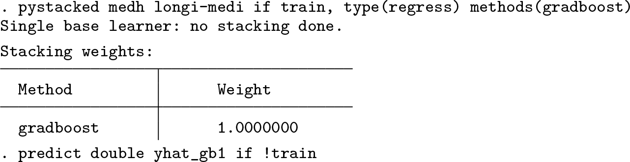
As a first example, we use pystacked to fit gradient-boosted regression trees and save the out-of-sample predicted values. Because we consider a regression task rather than a classification task, we specify type(regress) (but because this is the default, it could also be omitted). The option methods(gradboost) selects gradient boosting. We will later see that we can specify more than one learner in methods() and that we can also fit gradient-boosted classification trees.

The output shows the stacking weights associated with each base learner. Because we only consider one method, the output is not particularly informative and simply shows a weight of one for gradient boosting. Yet pystacked has fit 100 boosted trees (the default) in the background using scikit-learn’s ensemble.GradientBoosted- Regressor.

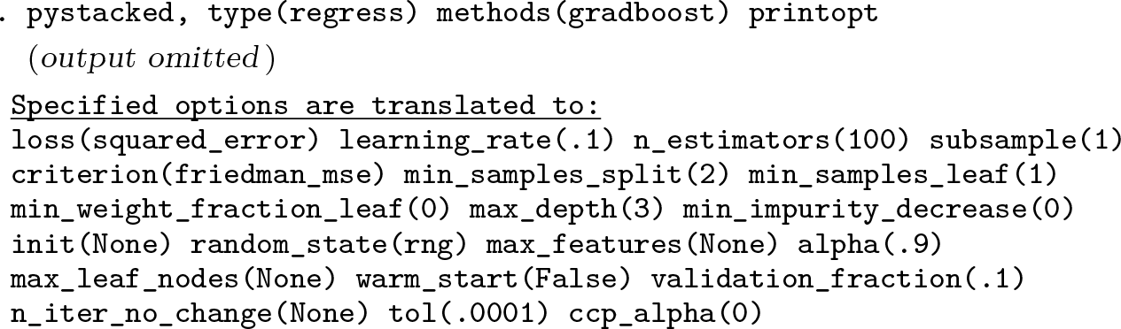
Before we tune our gradient boosting learner, we retrieve a list of available options. The default options for gradient boosting can be listed in the console, and the scikit-learn documentation provides more detail on the allowed parameters of each option.

We consider two additional specifications. Note that we restrict ourselves to a few selected specifications for illustrative purposes. We stress that careful parameter tuning should consider a grid of values across multiple learner parameters. The first specification reduces the learning rate from 0.1 (the default) to 0.01. The second specification reduces the learning rate and increases the number of trees from 100 (the default) to 1,000. We use cmdopt1() because gradient boosting is the first (and only) method listed in methods().

We can then compare the performance across the three models using the out-ofsample mean squared prediction error (MSPE):

The initial gradient booster achieves an out-of-sample MSPE of 29.87. The second gradient booster uses a reduced learning rate of 0.01 and performs much worse, with an MSPE of 71.10. The third gradient booster performs only slightly worse than the first, illustrating the tradeoff between the learning rate and the number of trees.

Pipelines

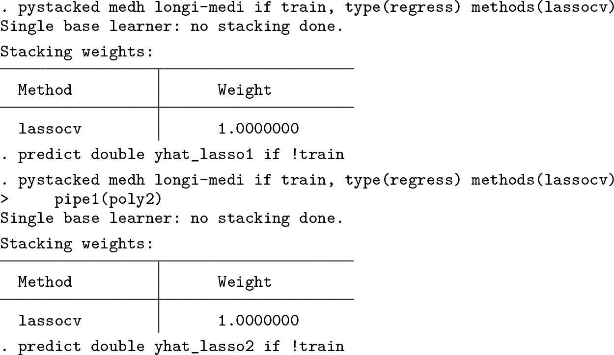
We can make use of pipelines to preprocess our predictors. This is especially useful in the context of stacking when we want to, for example, use second-order polynomials of predictors as inputs for one method but only use elementary predictors for another method. Here we compare lasso with and without the poly2 pipeline:

We could replace pipe1(poly2) with xvars1(c.(medh longi-medi)##c.(medh longi-medi)). In fact, the latter is more flexible and allows, for example, creation of interactions for some predictors and not for others.

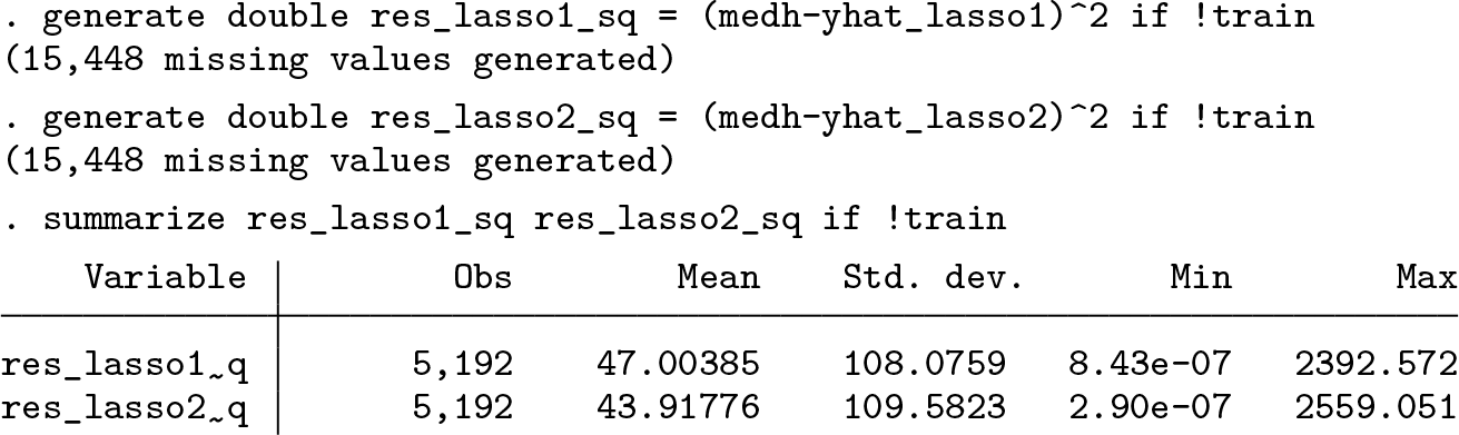
We again calculate the out-of-sample MSPE:

The poly2 pipeline improves the performance of the lasso, indicating that squared and interaction terms constitute important predictors. However, the lasso does not perform as well as gradient boosting in this application.

4.2 Stacking regression

We now consider a stacking regression application with five base learners: 1) linear regression, 2) lasso with penalty chosen by cross-validation, 3) lasso with second-order polynomials and interactions, 4) random forest with default settings, and 5) gradient boosting with a learning rate of 0.01 and 1,000 trees. That is, we use the lasso twice—once with and once without the poly2 pipeline. Indeed, nothing keeps us from using the same algorithm multiple times. This way, we can combine the same algorithm with different settings.

Note the numbering of the pipe∗ () and cmdopt∗ () options below. We apply the poly2 pipe to the third method ( lassocv). We also change the default learning rate and the number of estimators for gradient boosting (the fifth estimator).

The above syntax becomes a bit difficult to read with many methods and many options. pystacked‘s second syntax is easier to use with many base learners.

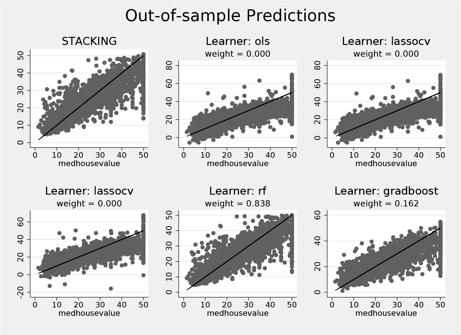
The stacking weights shown in the output determine how much each method contributes to the final stacking predictor. In this example, ordinary least squares and lasso based on both sets of predictors all receive a weight of zero. Random forest receives a weight of 83.8%, and gradient boosting contributes the remaining 16.2% of the weight to the final predictor.

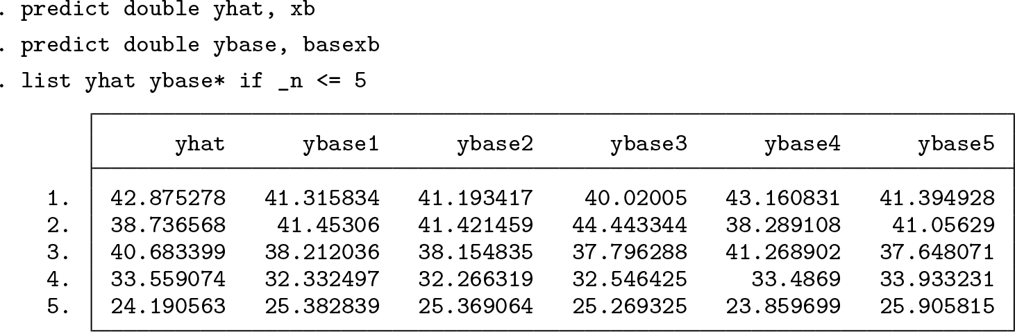
Predicted values

In addition to the stacking predicted values, we can also get the predicted values of each base learner using the basexb option:

Plotting

pystacked also comes with plotting features. The graph option creates a scatterplot of predicted values on the vertical and observed values on the horizontal axis for stacking and each base learner; see figure 1. The black line is a 45-degree line and shown for reference. Because pystacked with graph can be used as a postestimation command, there is no need to rerun the stacking estimation.

Figure 1.

Out-of-sample predicted values and observed values created using the graph option after stacking regression

Figure 1 shows the out-of-sample predicted values. To see the in-sample predicted values, simply omit the holdout option. Note that the holdout option will not work if the estimation was run on the whole sample.

RMSPE table

The table option allows comparing stacking weights with in-sample, cross-validated, and out-of-sample RMSPEs. As with the graph option, we can use table as a postestimation command:

4.3 Stacking classification

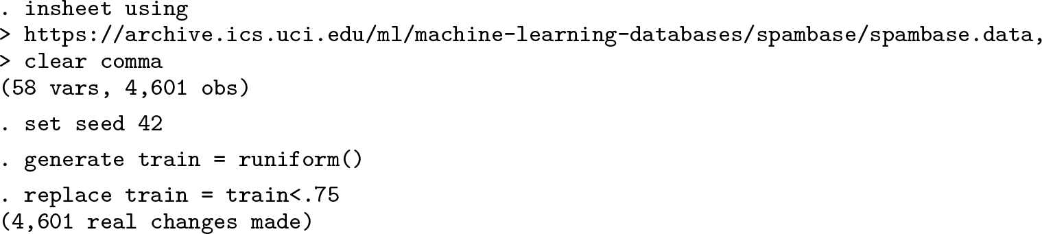
pystacked can be applied to binary classification problems. For demonstration, we consider the Spambase data of Cranor and LaMacchia (1998), which we retrieve from the UCI Machine Learning Repository. We load the data and split the data into training and validation samples using an approximate 75/25 split.

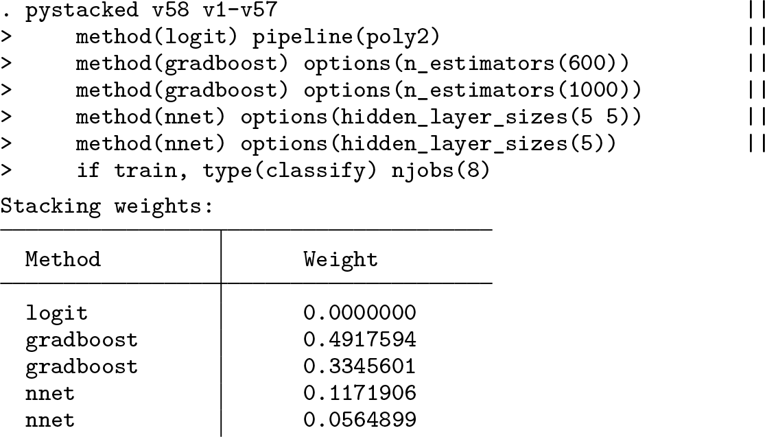
The example below is more complicated. We go through it step by step:

We use five base learners: logistic regression, two gradient boosters, and two neural nets.

We apply the poly2 pipeline to logistic regression, which creates squares and interaction terms of the predictors, but not to other methods.

We use gradient boosting with 600 and 1,000 classification trees.

We consider two specifications for the neural nets: one neural net with two hidden layers of five nodes each and another neural net with one hidden layer of five nodes.

Finally, we use type(classify) to specify that we are considering a classification task and njobs(8) switches parallelization on using 8 cores.

As in the previous regression example, gradient boosting receives the largest stacking weight and thus contributes most to the final stacking prediction.

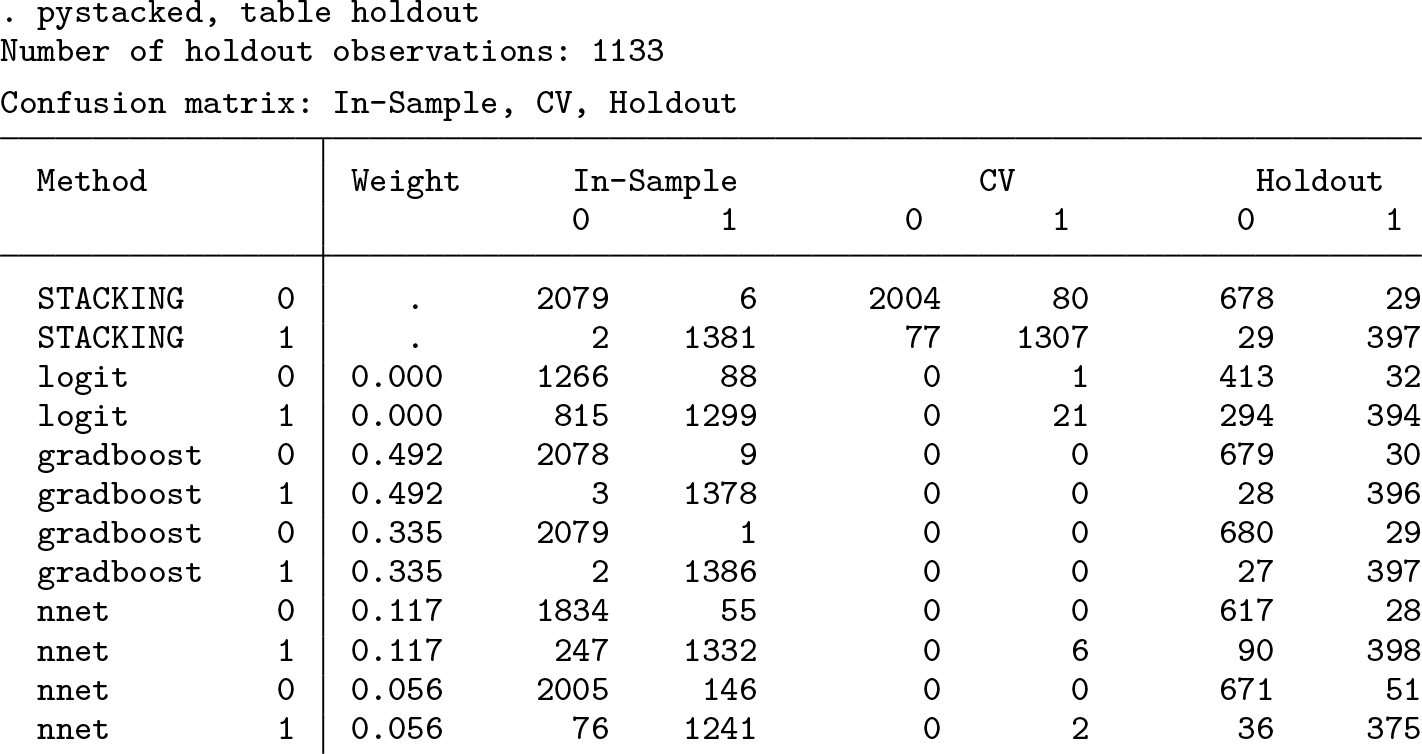
Confusion matrix

Confusion matrices allow comparing actual and predicted outcomes in a 2 × 2 matrix. pystacked provides a compact table format that combines confusion matrices for each base learner and for the final stacking classifier for both the training and the validation partitions.

For example, the table shows 29 false positives for stacking and 294 for logistic regression in the validation partition, while the number of false negatives is 29 and 32, respectively. The accuracy of stacking and logistic regression is thus given by (678 + 397)/1133 = 94.9% and (413 + 394)/1133 = 71.2%.

Plotting

pystacked supports ROC curves, which allow assessment of the classification performance for varying discrimination thresholds. The y axis in a ROC plot corresponds to sensitivity (true-positive rate), and the x axis corresponds to 1 − specificity (false-positive rate). The area under the curve displayed below each ROC plot is a common evaluation metric for classification problems.

Figure 2.

Out-of-sample ROC curves created using the graph option after stacking regression

5 Conclusion

In this article, we introduced the pystacked command. The command not only makes a range of popular supervised machine learners available, such as regularized regression, random forests, and gradient-boosted trees, but also facilitates combining multiple learners for stacking regression or classification. pystacked comes with several practically relevant features: for example, sparse matrix support, learner-specific predictors, pipelines for predictor transformations, and two alternative syntaxes. Nevertheless, we also see the potential for improvement in at least two directions. First, pystacked offers few diagnostics for individual learners. Features such as variable importance plots and coefficient estimates for parametric learners could be added in later versions.³ Second, the deep learning features of pystacked are currently relatively limited and could be improved by adding support for other deep learning algorithms.

7 Programs and supplemental material

Supplemental Material, sj-zip-1-stj-10.1177_1536867X231212426 - pystacked: Stacking generalization and machine learning in Stata

Supplemental Material, sj-zip-1-stj-10.1177_1536867X231212426 for pystacked: Stacking generalization and machine learning in Stata by Achim Ahrens, Christian B. Hansen and Mark E. Schaffer in The Stata Journal

References

1.
AhrensA.HansenC. B.SchafferM. E.. 2020. lassopack: Model selection and prediction with regularized regression in Stata. Stata Journal20: 176–235. https://doi.org/10.1177/1536867X20909697.
2.
AhrensA.HansenC. B.SchafferM. E.WiemannT.. 2023. ddml: Stata module for double/debiased machine learning. Statistical Software Components S459175, Department of Economics, Boston College. https://ideas.repec.org/c/boc/bocode/s459175.html.
3.
AhrensA.HansenC. B.SchafferM. E.WiemannT.. Forthcoming. ddml: Double/debiased machine learning in Stata. Stata Journal.
BuitinckL.LouppeG.BlondelM.PedregosaF.MüllerA.GriselO.NiculaeV., et al.2013. API design for machine learning software: Experiences from the scikitlearn project. European Conference on Machine Learning and Principles and Practices of Knowledge Discovery in Databases Workshop: Languages for Data Mining and Machine Learning.
FedorovaE.LedyaevaS.DrogovozP.NevredinovA.. 2022. Economic policy uncertainty and bankruptcy filings. International Review of Financial Analysis82: 102174. https://doi.org/10.1016/j.irfa.2022.102174.
GuentherN.SchonlauM.. 2018. svmachines: Stata module providing support vector machines for both classification and regression. Statistical Software Components S458564, Department of Economics, Boston College. https://ideas.repec.org/c/boc/bocode/s458564.html.
14.
HastieT.TibshiraniR.FriedmanJ.. 2009. The Elements of Statistical Learning: Data Mining, Inference, and Prediction. 2nd ed. New York: Springer. https://doi.org/10.1007/978-0-387-84858-7.
15.
HookerJ.DuveillerG.CescattiA.. 2018. A global dataset of air temperature derived from satellite remote sensing and weather stations. Scientific Data 5: 180246. https://doi.org/10.1038/sdata.2018.246.
LiangD.TsaiC.-F.LuH.-Y.ChangL.-S.. 2020. Combining corporate governance indicators with stacking ensembles for financial distress prediction. Journal of Business Research120: 137–146. https://doi.org/10.1016/j.jbusres.2020.07.052.
PedregosaF.VaroquauxG.GramfortA.MichelV.ThirionB.GriselO.BlondelM., et al.2011. Scikit-learn: Machine learning in Python. Journal of Machine Learning Research12: 2825–2830. https://doi.org/10.48550/arXiv.1201.0490.
van der LaanM. J.PolleyE. C.HubbardA. E.. 2007. Super learner. Statistical Applications in Genetics and Molecular Biology 6. https://doi.org/10.2202/1544-6115.1309.
24.
van der LaanM. J.RoseS.. 2011. Targeted Learning: Causal Inference for Observational and Experimental Data. New York: Springer. https://doi.org/10.1007/978-1-4419-9782-1.