Sage Journals: Discover world-class research

Abstract

In this article, we introduce a new command, clan, that conducts a cluster-level analysis of cluster randomized trials. The command simplifies adjusting for individual- and cluster-level covariates and can also account for a stratified design. It can be used to analyze a continuous, binary, or rate outcome.

Keywords

st0727 clan few clusters analysis method adjusting for covariates stratified trial group randomized trial cluster randomized trial cluster summary analysis

1 Introduction

A cluster randomized controlled trial (CRT), also known as a group randomized trial, is an experimental study design commonly used, for example, in health, social science, policy, and education research. In CRTs, the unit of randomization consists of a group of individuals. For example, it could be a hospital, geographical area, or school (each constituting a “cluster”), with the clusters, rather than individuals, randomly allocated to different interventions.

Statistical analysis must account for the correlation among individuals within the same cluster, which can be achieved using individual data analysis methods such as generalized linear mixed models, generalized estimating equations, or cluster–robust standard errors with a generalized linear model. Alternatively, it can be achieved by collapsing the data to summary statistics for each cluster, which is known as a clusterlevel analysis or sometimes a cluster-summary analysis. In addition, the number of randomization units (clusters) is often small; a recent review of medical journals found a median of 25 clusters (Kahan et al. 2016) per trial. There is a need for methods that can provide robust inference even with a small number of clusters. This also increases the risk of a chance imbalance in potential confounders between the arms, and adjustment of potential confounders in the analysis becomes important.

Here we introduce a command for cluster-level analysis. Individual-level data are summarized for each cluster, and simple independent data analysis methods can be used on these summaries. The method can be used with continuous, binary, incidencerate, and ordinal outcomes. It has been found to perform well in a range of scenarios, including nonnormality of cluster-level means and with a small number of clusters (Gail et al. 1996; Bennett et al. 2002; Thompson et al. 2022; Ukoumunne, Carlin, and Gulliford 2007).

There are several advantages to this method over individual-level methods. Clusterlevel analysis is known to maintain type-one error with as few as 4 clusters in total, whereas individual-level methods have inflated type-one errors with as many as 40 clusters and require small-sample corrections that have variable success (Leyrat et al. 2018; Thompson et al. 2022). Another advantage is the ease of calculating a risk ratio for a binary outcome when some individual-level methods struggle with convergence (Blizzard and Hosmer 2006). Last, a cluster-level analysis is the only known way to account for a matched-pairs trial design in the analysis of a binary or incidence-rate outcome (Hayes and Moulton 2017).

However, the method is not without limitations. Unweighted cluster-level analysis can be less efficient than an individual-level analysis when cluster size varies and there are many clusters (Thompson et al. 2022). Weighted cluster-level analysis using weighted least squares or a weighted t test has been proposed to improve the method efficiency, but difficulties incorporating uncertainty in the weights generally lead to standard errors that are too small and have inflated type-one errors (Westgate 2013). In addition, adjusting for individual-level covariates becomes more difficult; it requires several steps before the data are summarized by cluster (Bennett et al. 2002).

In this article, we introduce the clan command, which simplifies implementation of cluster-level analysis. We will begin by describing the analysis method before presenting our command. We provide several illustrative examples and finish with some conclusions.

2 Statistical methods

clan performs a cluster-level analysis either unadjusted or adjusting for individual- and cluster-level covariates. It can be used with binary, incidence-rate (events per persontime), and continuous outcomes. It can also be used to account for a stratified design. Depending on the type of outcome being analyzed, different intervention effect measures may be of interest. For a binary outcome, we may be interested in the risk difference or the risk ratio. For an incidence-rate outcome, we may be interested in the incidencerate difference or incidence-rate ratio. For a continuous outcome, the most common intervention effect of interest is a difference in the mean of the outcome.

In this section, we provide the technical details of this method as proposed by Bennett et al. (2002) and Hayes and Moulton (2017).

2.1 Unadjusted analysis: Calculating intervention effects

We define y_ijk as the observed outcome of individual k = 1,…, m_ij in cluster j = 1,…, C_i in arm i = 0, 1 for control and intervention, respectively, where C_i is the number of clusters in arm i and m_ij is the number of individuals in cluster j in arm i. For example, y_ijk could be the body mass index (BMI) of student k in school j, receiving a diet program i. For each individual, we define n_ijk as the person follow-up time of person k in cluster j in arm i for rate outcomes and set n_ijk = 1 for continuous and binary outcomes.

We begin by calculating a summary statistic of the outcome for each cluster j and arm i as the sum of the observed outcomes divided by the cluster size:

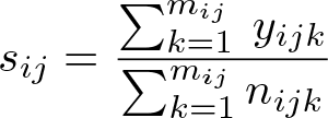
s_{i j} = \frac{\sum_{k = 1}^{m_{i j}} y_{i j k}}{\sum_{k = 1}^{m_{i j}} n_{i j k}}

In each cluster, this gives the risk (or proportion or prevalence) for a binary outcome, the incidence rate (number of events per person-time) for a rate outcome, or the mean for a continuous outcome. In our diet program example, s_ij would correspond to the average BMI observed in school j in arm i.

2.1.1 Absolute effect size: Risk difference, rate difference, and mean difference

The risk, incidence rate, or mean in each arm i can be estimated by the arithmetic mean of the cluster-summary statistics for the clusters in that arm:

{\bar{s}}_{i} = \frac{1}{C_{i}} \sum_{j = 1}^{C_{i}} s_{i j}

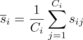
In our diet program example, this would correspond to the mean of the average BMIs across the schools in arm i. Note that each cluster is here given an equal weight.

The unadjusted absolute effect can then be estimated by the difference of these arithmetic means between the intervention and control arm:

{\bar{s}}_{1} - {\bar{s}}_{0}

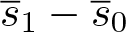
This could be derived arithmetically or, equivalently, using an ordinary least-squares regression. This is the approach used in clan to facilitate the estimation of the variance and to conduct inference as shown below.

The following linear model is fit to the cluster-level summary statistics,

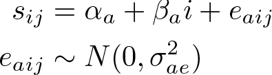
\begin{array}{l} s_{i j} = α_{a} + β_{a} i + e_{a i j} \\ e_{a i j} ~ N (0, σ_{a e}^{2}) \end{array}

where the a index indicates parameters for the absolute effect model; α_a is the intercept corresponding to the mean of the cluster-level statistics in the control arm, ${\bar{s}}_{0}$ ; β_a is the slope capturing the difference between the intervention and control means, ${\bar{s}}_{1} - {\bar{s}}_{0}$ ; and e_aij are independent, normally distributed random errors.

For risk or rate outcomes, the assumption of normality may be violated, but the method is typically robust to this nonnormality (Bennett et al. 2002).

In our diet program example, α_a is the arithmetic mean of the school-mean BMIs in the control arm, and β_a is the difference in the mean BMI between the two diet programs.

2.1.2 Relative effect size: Risk ratio and incidence-rate ratio

The risk ratio and incidence-rate ratio are both examples of relative intervention effects. For relative effects, we use the natural logarithms of the cluster summaries. This facilitates calculation and inference of ratio measures as described below. We can estimate the risk or rate in each arm by the geometric mean of the cluster summaries:

{\bar{s}}_{G i} = \exp {\frac{1}{C_{i}} \sum_{j = 1}^{C_{i}} \ln (s_{i j})}

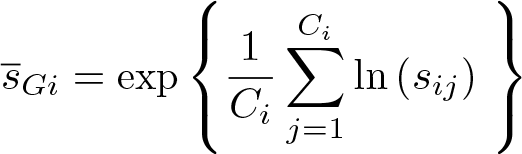
These geometric means are displayed in the output of clan for each arm if a ratio effect is requested. The geometric mean is often preferable to arithmetic means for skewed data because it is less strongly influenced by outliers (Alexander 2012). Risks and rates with low prevalence are often skewed because their distribution is bounded by zero and the log of the cluster-level risks and rates are likely to be closer to a normal distribution than the untransformed values.

The unadjusted risk or incidence-rate ratio can be estimated as the ratio of these geometric means in the intervention and control arms:

\frac{{\bar{s}}_{G 1}}{{\bar{s}}_{G 0}}

As with the absolute effect, we can estimate this relative effect arithmetically or using ordinary least squares. This time, the linear model is fit to the logarithm of the clustersummary statistics,

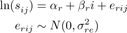
\begin{array}{l} \ln (s_{i j}) = α_{r} + β_{r} i + e_{r i j} \\ e_{r i j} ~ N (0, σ_{r e}^{2}) \end{array}

where the r index is used to indicate parameters for the relative effect model; α_r is the intercept corresponding to the logarithm of the geometric mean in the control arm ln $({\bar{s}}_{G 0})$ ; β_r is the slope corresponding to the natural logarithm of the ratio of the geometric means, ln $({\bar{s}}_{G 1} / {\bar{s}}_{G 0})$ ; and e_rij are independent, normally distributed random errors.

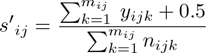
Because we use logarithms in this method, the relative effect size estimator is not defined if any cluster has no events $(\sum_{k = 1}^{m_{i j}} y_{i j k} = 0)$ . Several solutions have been 2017; Habib 2012; Alexander et al. 2005). In clan, if any clusters meet this condition, we add half an event to every cluster (Hayes and Moulton 2017; Breslow 1981), giving the following alternative cluster-summary statistic for every cluster:

{s^{'}}_{i j} = \frac{\sum_{k = 1}^{m_{i j}} y_{i j k} + 0.5}{\sum_{k = 1}^{m_{i j}} n_{i j k}}

We then substitute s′_ij for s_ij in the calculations above.

2.2 Unadjusted analysis: p-value and confidence interval

We calculate p-values using Wald tests of the ordinary least-squares regression estimate of the intervention effect coefficient with the variance of the coefficient estimate estimated using standard formulas for ordinary least squares.

For an absolute effect, the p-value for the statistical test H ₀ : $\hat{β_{a}} = 0$ is taken from the t distribution with C ₀ + C ₁ − 2 degrees of freedom (DF)

\frac{{\hat{β}}_{a}}{\sqrt{\hat{Var} ({\hat{β}}_{a})}} ~ t_{C_{0} + C_{1} - 2}

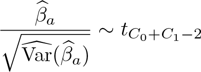
and 95% confidence intervals (CIs) are calculated as ${\hat{β}}_{a} \pm t_{C_{0} + C_{1} - 2, 0.025} \sqrt{\hat{Var} ({\hat{β}}_{a})}$ , where t _DF _,q indicates the value of the t distribution with DF and an inverse cumulative probability of q.

For the relative effect, calculations are similar. The p-value is taken from the t distribution

\frac{{\hat{β}}_{r}}{\sqrt{\hat{Var} ({\hat{β}}_{r})}} ~ t_{C_{0} + C_{1} - 2}

and CIs are calculated as $\exp {{\hat{β}}_{r} \pm t_{C_{0} + C_{1} - 2, 0.025} \sqrt{\hat{Var} ({\hat{β}}_{r})}}$

2.3 Adjusted analysis: Estimating the intervention effect

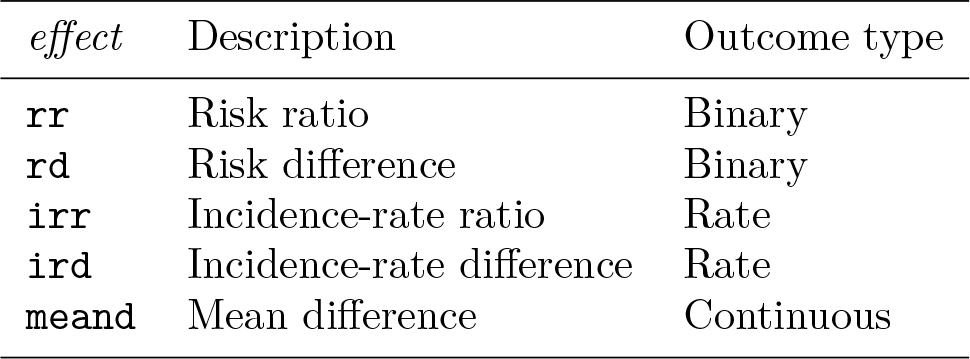
Adjusting for individual-level covariates is done in a two-stage approach. First, we estimate a cluster-summary residual for each cluster, and second, we analyze these residuals. The process is summarized for each intervention effect measure in table 1.

Table 1.

Summary of steps to calculate each adjusted intervention effect measure

	Risk difference	Risk ratio	Incidence-rate difference	Incidence-rate ratio	Mean difference
Outcome type	Binary	Binary	Event per person-time	Event per person-time	Continuous outcome
Interpretation of cluster-summary measure s_ij	Risk	Risk	Rate	Rate	Mean
Unadjusted effect estimate	${\bar{s}}_{1} - {\bar{s}}_{0}$	${\bar{s}}_{G 1} / {\bar{s}}_{G 0}$	${\bar{s}}_{1} - {\bar{s}}_{0}$	${\bar{s}}_{G 1} / {\bar{s}}_{G 0}$	${\bar{s}}_{1} - {\bar{s}}_{0}$
Stage one: regression of individual outcomes on covariates	Logistic regression	Logistic regression	Poisson regression	Poisson regression	Linear regression
Predicted outcome µ_ijk	Probability of individual having the outcome	Probability of individual having the outcome	Expected number of events in individual’s follow-up time	Expected number of events in individual’s follow-up time	Estimated mean outcome
Residual	Difference residual	Ratio residual	Difference residual	Ratio residual	Difference residual
Stage two: regression of residuals on arm	Linear regression of difference residual	Linear regression of logarithm of ratio residual	Linear regression of difference residual	Linear regression of logarithm of ratio residual	Linear regression of difference residual

2.3.1 Stage one: Calculating cluster-summary residuals

A. Fit regression of outcome on covariates

In the first stage, we regress the outcome on the adjustment covariates, ignoring clustering and the trial arm. We use a generalized linear model,

g (μ_{i j k}) = \ln (n_{i j k}) + \sum_{l} γ_{l} z_{i j k l}

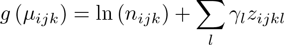
where g is the link function: the logit function for a binary outcome, the logarithm function for a rate outcome, and the identity function for a continuous outcome. µ_ijk is the expected outcome of individual k in cluster j in arm i and is assumed to follow a binomial distribution for a binary outcome, a Poisson distribution for an incidence-rate outcome, and a normal distribution for a continuous outcome. γ_l is a coefficient for the lth covariate, and z_ijkl is the value of the lth covariate for individual k in cluster j in arm i. ln(n_ijk ) is an offset that equals zero for binary and continuous outcomes because n_ijk = 1 for these outcomes.

B. Predict outcomes

From this regression model, we predict the expected outcome for each individual, µ_ijk . For a binary outcome, this is a predicted probability of the outcome. For a rate outcome, this is the expected number of events in each individual’s follow-up time. For a continuous outcome, this is the expected value of the outcome.

C. Calculate residuals

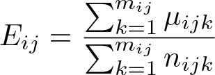
For each cluster, we then calculate the observed cluster-summary statistics s_ij (defined in section 2.1) and cluster-summary statistics for expected outcomes, which are defined as

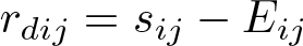
E_{i j} = \frac{\sum_{k = 1}^{m_{i j}} μ_{i j k}}{\sum_{k = 1}^{m_{i j}} n_{i j k}}

From these, we calculate residuals for each cluster. If we plan to estimate an absolute effect (risk difference, rate difference, mean difference), we calculate a difference residual:

r_{d i j} = s_{i j} - E_{i j}

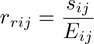
If we plan to estimate a relative effect (risk ratio, rate ratio), we calculate a ratio residual:

r_{r i j} = \frac{s_{i j}}{E_{i j}}

2.3.2 Stage two: Analyze the residuals

These cluster-level residuals become our new unit of comparison between the clusters. Inference is conducted by substituting r_dij or r_rij for s_ij in section 2.1.

2.4 Adjusted analysis: p-value and CI

The p-value for the intervention effect is calculated using a Wald test from the second stage regression using the same methods as the unadjusted analysis, with r_dij or r_rij substituted for s_ij .

The DF are recalculated to account for adjustment of any cluster-level covariates. This is because the stage-2 regression model is on cluster-level data, and any adjustment for cluster-level variables at stage 1 imposes linear constraints on the cluster-level parameters (while adjustment for individual-level variables does not). We reduce the DF by P, the number of parameters corresponding to these cluster-level covariates in the first-stage regression. The DF are then calculated as

DF = C_{0} + C_{1} - 2 - P

clan detects cluster-level covariates by identifying adjustment variables that are constant within clusters. For factor variables, each factor value is assessed separately: this means that some categories can be counted as cluster level (if the factor indicator is either 0 or 1 in any given cluster), while others may be counted as individual level (if the factor indicator varies within some clusters) with a maximum number of cluster-level factors equal to the number of factor values minus one.

2.5 Accounting for stratified randomization

Stratified randomization can be used to ensure balance of key characteristics between the arms of the trial. Strata are created with similar values of these characteristics, and randomization is implemented ensuring an equal number of clusters in each arm within the strata. Accounting for the stratification in the analysis is recommended because it can greatly improve precision (Hayes and Moulton 2017).

In the clan command, the categorical variable defining the strata is included as a covariate in the first-stage regression that calculates expected outcomes of the analysis adjusted for other covariates and the second-stage regression that estimates the intervention effect for both adjusted and unadjusted analysis. The DF are reduced by one less than the number of strata: DF = C ₀ + C ₁ − 2 − P − (S − 1), where S is the number of strata.

3 The clan command

The syntax of the clan command is explained below. In addition to implementation of the method, we provide an option to plot or save the cluster summaries.

3.1 Syntax

clan depvar [indepvars] [if] [in], arm( varname ) cluster( varname ) effect( effect ) [ fuptime( varname[, per( # )]) strata( varname ) plot saving( filename [, replace]) level( # )]

depvar is the dependent variable and indepvars are the adjustment covariates.

3.2 Options

arm( varname ) specifies the numeric variable that defines the trial arm. It must be coded as 0 or 1. arm() is required.

cluster( varname ) specifies the numeric variable that defines the clusters. cluster() is required.

effect( effect ) specifies the measure of effect to calculate. effect() is required. effect may be one of the following:

effect	Description	Outcome type
rr	Risk ratio	Binary
rd	Risk	difference Binary
irr	Incidence-rate ratio	Rate
ird	Incidence-rate difference	Rate
meand	Mean difference	Continuous

rd, ird, and meand are absolute effects. rr and irr are relative effects, as described in section 2.

fuptime( varname [, per( # )])specifies the numeric variable that defines the length of time each participant was in the study; this is required when either rate differences or ratios are to be calculated. There is also an option to specify different units when displaying the incidence rates.

strata( varname ) specifies the numeric variable that defines the stratification used in the trial randomization. Only one stratification factor is permitted. It must be constant within clusters.

plot produces a scatterplot of the cluster-level summaries used to produce the effect measure. For adjusted analyses, these will be residual values and hence will not have a direct interpretation.

saving( filename [, replace]) saves a dataset with the cluster-level summaries. A new filename is required unless replace is also specified. replace allows the filename to be overwritten with new data.

level( # ) specifies the confidence level, as a percentage, for CIs. The default is level(95) or as set by set level.

3.3 Illustrative examples

We will now illustrate the use of the clan command using three examples used in the book Cluster Randomized Trials (Hayes and Moulton 2017). These trials are discussed in more detail in the book and the corresponding publications.

3.4 Binary outcome

To demonstrate the use of the clan command on a binary outcome, we will use data from the MkV trial. MkV was a cluster-randomized trial evaluating an adolescent sexual health program in Mwanza, Tanzania (Ross et al. 2007; Hayes et al. 2005). It randomly allocated 20 communities (geographical areas) to receive the intervention, an integrated adolescent sexual health program, or act as control. The randomization was stratified by HIV risk strata (high, medium, low). A cohort of students was followed up, and sexual health outcomes, including HIV status and knowledge about transmission of HIV, were collected at three years. We will focus on the analysis of the HIV knowledge outcome in boys. HIV knowledge was a binary outcome, where “good knowledge” was defined by correctly answering three questions about HIV transmission.

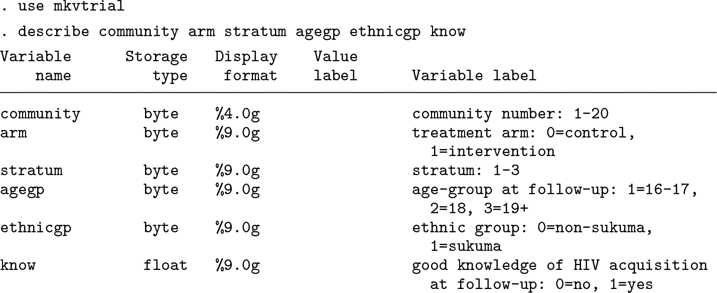
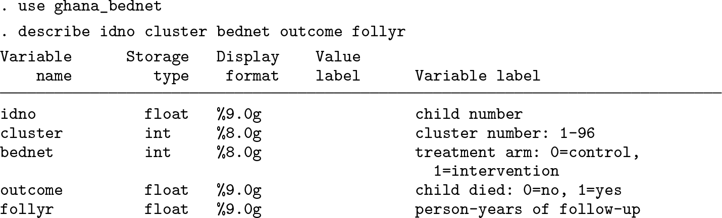
The dataset is described below:

The HIV knowledge outcome in each cluster is summarized in table 2.

Table 2.

Proportion of children with good HIV knowledge in each cluster of the MkV trial

Stratum	Control communities	Intervention communities
High risk	110/226 (48.7%)	164/204 (80.4%)
	65/171 (38.0%)	141/206 (68.4%)
	69/178 (38.8%)	111/171 (64.9%)
Medium risk	87/194 (44.8%)	139/219 (63.5%)
	102/229 (44.5%)	115/207 (55.6%)
	84/243 (34.6%)	172/237 (72.6%)
	121/196 (61.7%)	111/187 (59.4%)
Low risk	101/226 (44.7%)	119/169 (70.4%)
	102/175 (58.3%)	157/219 (71.7%)
	67/186 (36.0%)	127/257 (49.4%)

We can estimate the risk ratio between the trial arms using clan as follows:

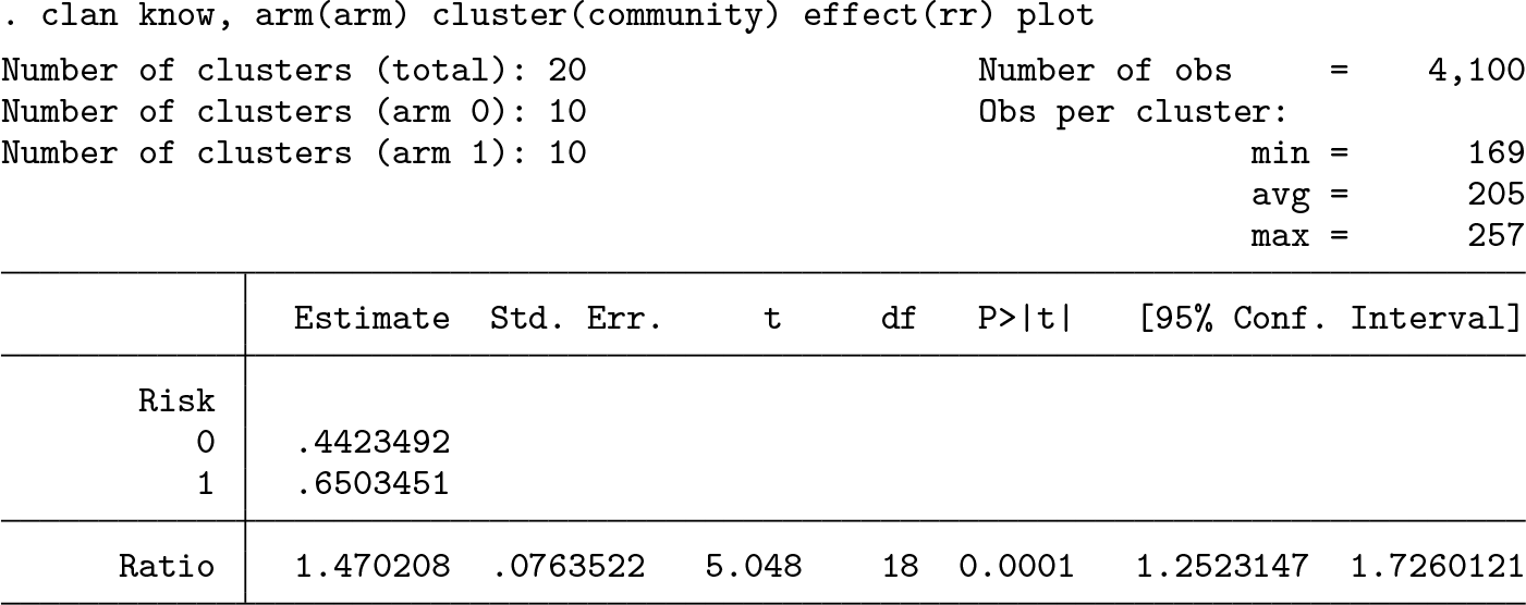
In the control clusters (arm = 0), an estimated 44.2% of students had a good knowledge of HIV acquisition compared with 65.0% in the intervention clusters (arm = 1). There was evidence of better knowledge in the intervention arm, with a rate ratio of 1.47 (95% CI: [1.25 to 1.73], p-value = 0.0001).

Because the effect measure is a ratio, the risk estimates are based on the geometric means of the cluster-level risks. The test statistic follows a t distribution with 18 DF (the number of clusters minus two).

The output also indicates the number of clusters and the number of observations in each cluster.

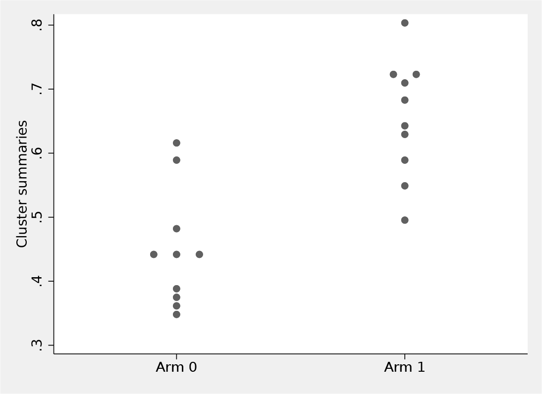
Inclusion of the plot option produces figure 1, which shows the cluster summaries by arm.

Figure 1.

Plot of cluster-level summaries (proportion of good HIV knowledge) by arm

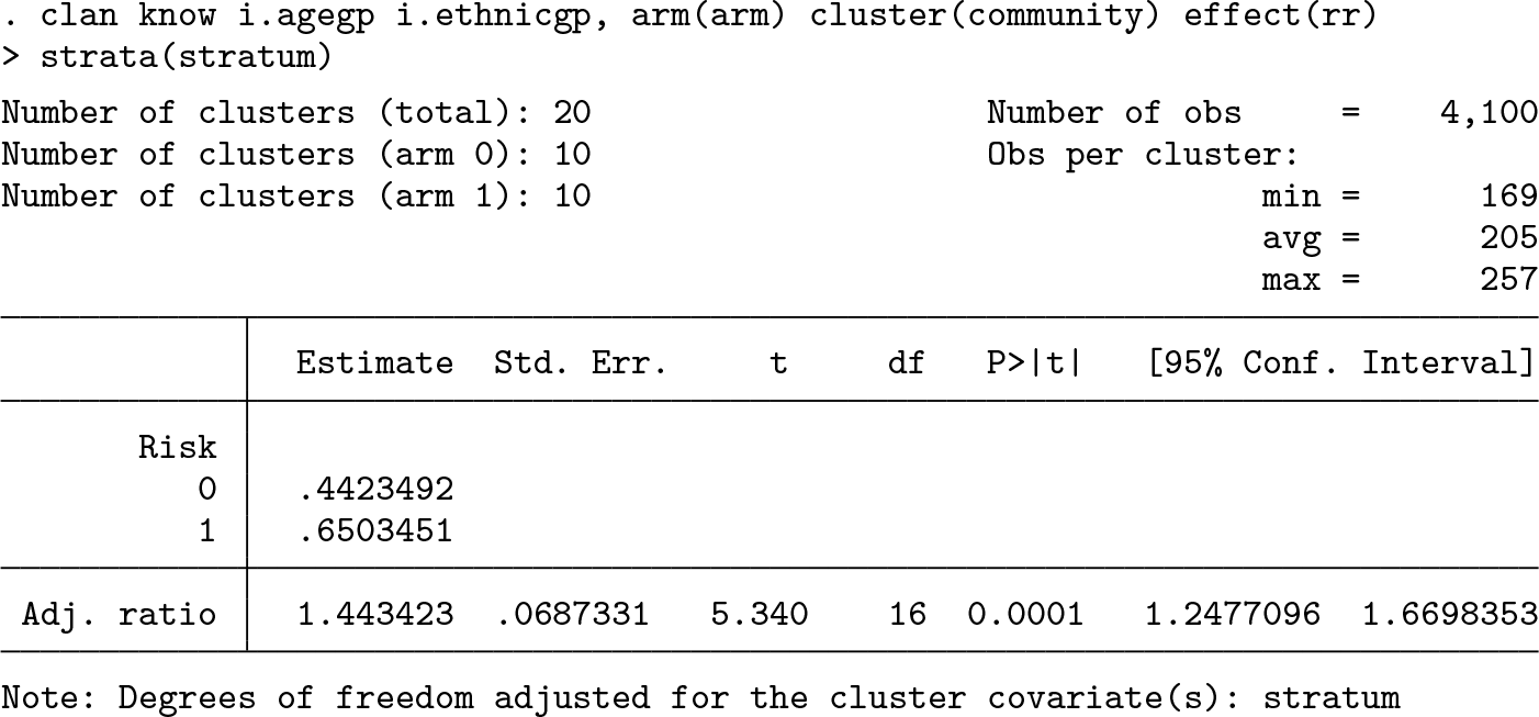
We may wish to adjust for baseline covariates (agegp and ethnicgp) and account for the stratification factor (stratum):

After we adjust for age group, ethnicity and strata, the risk ratio is 1.44 (95% CI: [1.25 to 1.67]). The DF were reduced by two to account for the cluster-level stratum variable, with three categories. Adjusting for individual-level variables (such as age and ethnicity) does not affect the DF.

3.5 Rate outcome

Binka et al. (1996) conducted a CRT to measure the impact of insecticide-impregnated bednets on child mortality in Northern Ghana. The study area was divided into 96 geographical clusters, and 48 were randomly selected to receive impregnated bednets while the remaining 48 acted as controls. A demographic surveillance system was set up to record births, deaths, and migration for two years. The dataset contains data on children aged 6–59 months at the beginning of the trial and shows their person-years of follow-up and whether the child died during follow-up.

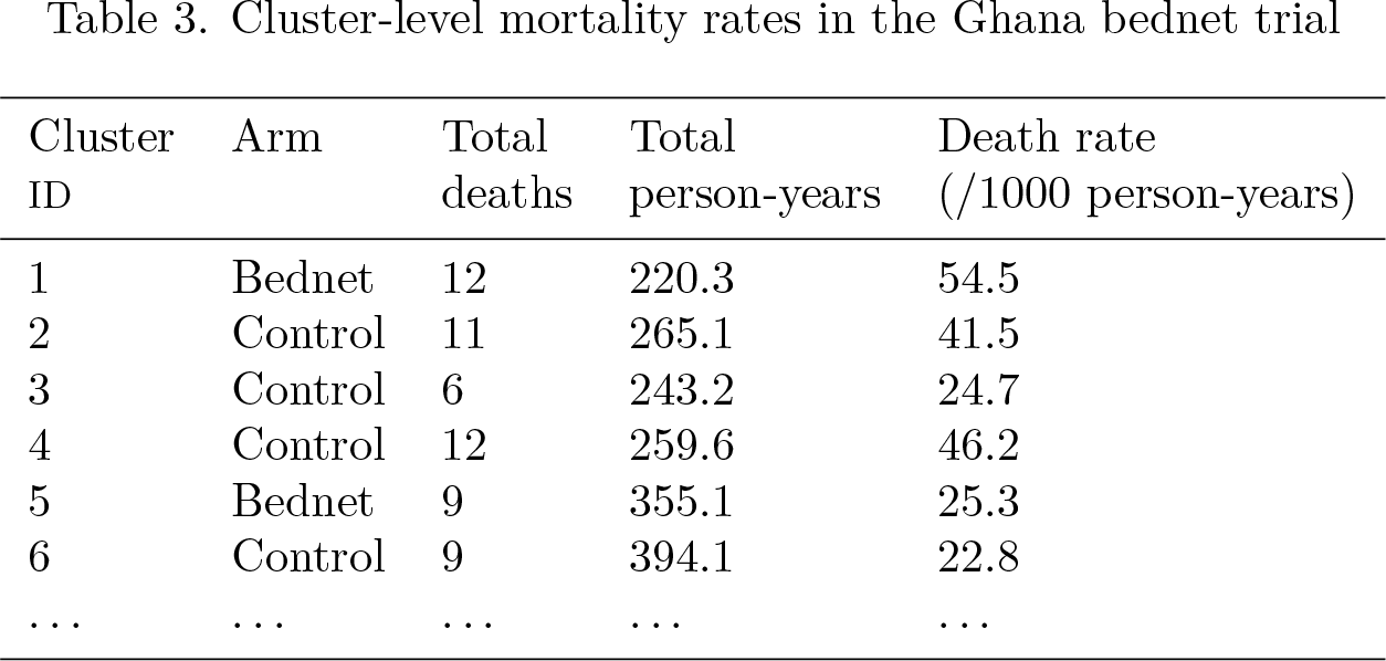
The primary trial outcome was all-cause mortality in children. Table 3 summarizes the total number of deaths, person-years of follow-up, and mortality rate for the first six clusters.

Table 3.

Cluster-level mortality rates in the Ghana bednet trial

Cluster ID	Arm	Total deaths	Total person-years	Death rate (/1000 person-years)
1	Bednet	12	220.3	54.5
2	Control	11	265.1	41.5
3	Control	6	243.2	24.7
4	Control	12	259.6	46.2
5	Bednet	9	355.1	25.3
6	Control	9	394.1	22.8
…	…	…	…	…

We can estimate the rate ratio between arms using the clan command:

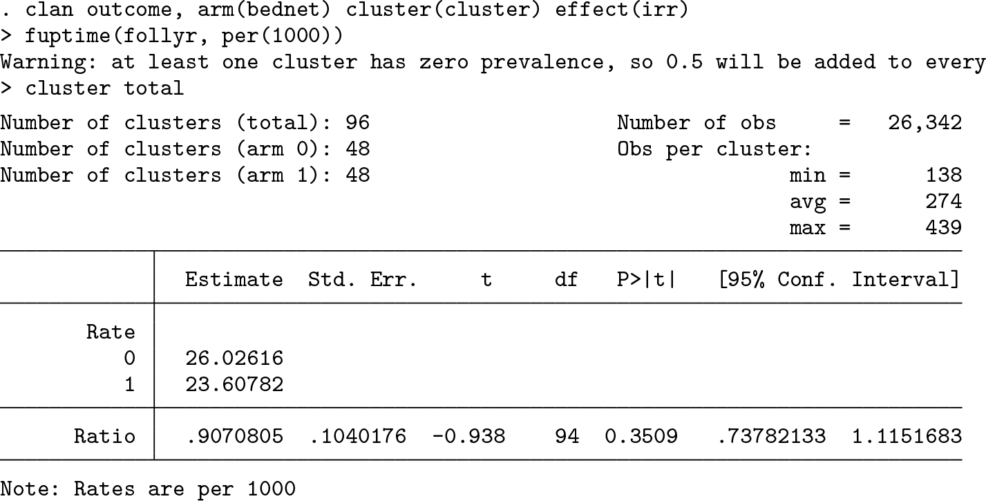
In the control clusters, there was an average of 26.0 deaths for each 1,000 person-years of follow-up, while in the bednet clusters, this rate was around 23.6 per 1,000 personyears. This corresponds to a rate ratio of 0.91 (95% CI: [0.74 to 1.11], p-value=0.35).

A warning message indicates that because one cluster has no events, a 0.5 event was added to each cluster before calculating the log-rate.

3.6 Continuous outcome

The SHARE trial aimed to improve sexual health knowledge through a school-based sexual health program in Scotland (Wight et al. 2002). A total of 25 secondary schools were randomly allocated to the intervention or control arms, and a measure of sexual health knowledge, −8 (poor knowledge) to 8 (good knowledge), was measured through a questionnaire two years later. The analysis was conducted separately for boys and girls, and we focus here on the analysis in the boys.

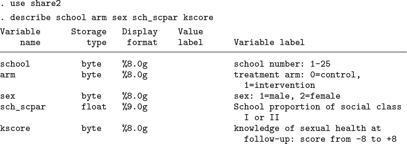
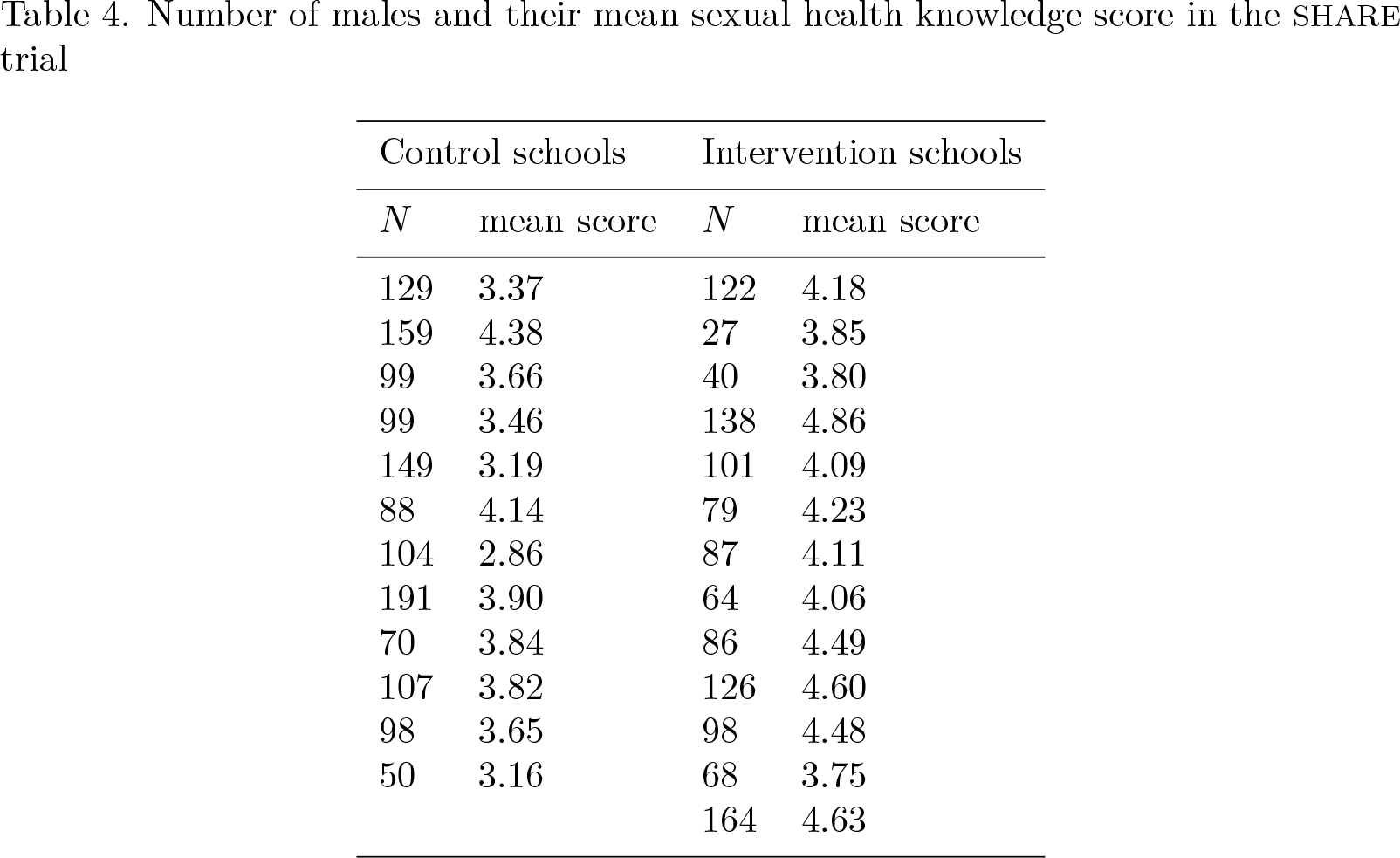
Table 4 shows the number of male respondents and their mean sexual health knowledge score for each of the 25 schools:

Table 4.

Number of males and their mean sexual health knowledge score in the SHARE trial

Control schools		Intervention schools
N	mean score	N	mean score
129	3.37	122	4.18
159	4.38	27	3.85
99	3.66	40	3.80
99	3.46	138	4.86
149	3.19	101	4.09
88	4.14	79	4.23
104	2.86	87	4.11
191	3.90	64	4.06
70	3.84	86	4.49
107	3.82	126	4.60
98	3.65	98	4.48
50	3.16	68	3.75
		164	4.63

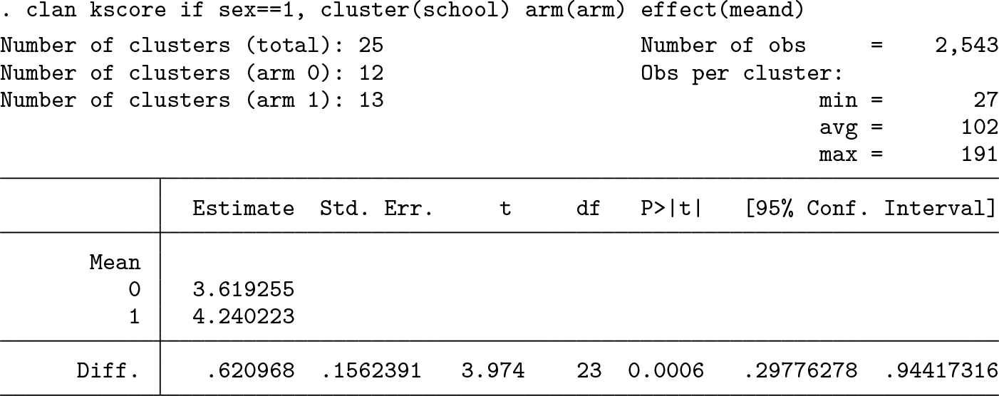
We can use clan to compare the mean knowledge score in boys between the two arms:

The average knowledge score for boys was 3.62 in the control schools compared with 4.24 in the intervention schools.

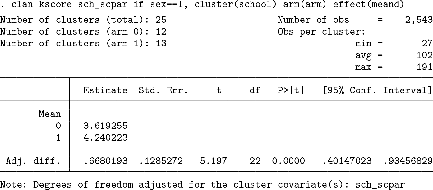
We can also estimate the mean difference adjusted for sch_scpar, a measure of social class distribution in each school:

Because social class is a cluster-level variable, 1 degree of freedom was lost. After adjustment, the mean difference in knowledge score between the two arms was 0.67 (95% CI: [0.40 to 0.93], p-value < 0.0001).

3.7 Conclusions

The clan command simplifies the analysis of CRTs using a cluster-level analysis. The command enables users to adjust for individual- and cluster-level covariates, account for the trial design, estimate relative and absolute effects, and plot their results. It can be used with binary, incidence-rate, or continuous outcomes.

There are some general limitations of the cluster-level analysis method and potential for further developments that should be considered when using clan. Calculation of relative effect sizes for risks and incidence rates is done by taking the logarithm of the cluster summaries. This raises two concerns: clusters with no events become difficult to handle, and the resulting ratio is a different estimand of a ratio of geometric means rather than a ratio of arithmetic means. To allow calculation of the logarithm of clusters with zero events, clan adds half an event to every cluster. However, this is known to bias the within-arm risk estimates and the intervention effect, particularly when clusters are small. There is a need for further work in validating alternative correction method that could be added to the command. The issue of geometric means is more complex. Some believe geometric means give a better measure of centrality in highly skewed data, which is often the case for low risks and incidence rates (Alexander et al. 2005). However, others have argued that arithmetic means could be more representative of the expected “population-average” effect. Estimating the variance of the arithmetic mean ratio is less straightforward than working on the logarithmic scale and would require further research to, for example, account for a stratified design. Future developments to clan should explore alternative estimators for these relative measures.

While the validity of the cluster-level analysis is well studied for both adjusted and unadjusted analyses (Bennett et al. 2002; Ukoumunne, Carlin, and Gulliford 2007) and unadjusted analyses have been compared with individual-level analysis (Leyrat et al. 2018; Thompson et al. 2022), there is a need for comparisons of the adjusted clusterlevel analysis method to individual-level analysis methods to ascertain the difference in power.

Future developments of the clan command could include estimation of a measure of between-cluster variability as required by CONSORT guidelines (Campbell et al. 2012), such as an intracluster correlation coefficient or coefficient of variation, and analysis of effect modification. We also plan to consider other effect measures such as odds ratios, allowing weights to be specified for each cluster, and accounting for a matched design.

This command will facilitate the conduct of cluster-level analysis of CRTs and encourage more widespread use of this robust approach.

5 Programs and supplemental materials

Supplemental Material, sj-zip-1-stj-10.1177_1536867X231196294 - Cluster randomized controlled trial analysis at the cluster level: The clan command

Supplemental Material, sj-zip-1-stj-10.1177_1536867X231196294 for Cluster randomized controlled trial analysis at the cluster level: The clan command by Jennifer A. Thompson, Baptiste Leurent, Stephen Nash, Lawrence H. Moulton and Richard J. Hayes in The Stata Journal

Footnotes

4 Acknowledgments

J. A. Thompson, B. Leurent, S. Nash, and R. J. Hayes are funded by the U.K. Medical Research Council (MRC) and the U.K. Department for International Development (DFID) under the MRC/DFID Concordat agreement and also part of the EDCTP2 programme supported by the European Union (grant ref: MR/R010161/1).

5 Programs and supplemental materials

To install a snapshot of the corresponding software files as they existed at the time of publication of this article, type

For the latest version of the clan command, type

References

Alexander

2012. Analysis of parasite and other skewed counts. Tropical Medicine and International Health 17: 684–693. https://doi.org/10.1111/j.1365-3156.2012.02987.x.

Alexander

N. D. E.

Solomon

A. W.

Holland

M. J.

Bailey

R. L.

West

S. K.

Shao

J. F.

Mabey

D. C. W.

Foster

. 2005. An index of community ocular Chlamydia trachomatis load for control of trachoma. Transactions of The Royal Society of Tropical Medicine and Hygiene 99: 175–177. https://doi.org/10.1016/j.trstmh.2004.05.003.

Bennett

Parpia

Hayes

Cousens

. 2002. Methods for the analysis of incidence rates in cluster randomized trials. International Journal of Epidemiology 31: 839–846. https://doi.org/10.1093/ije/31.4.839.

Binka

F. N.

Kubaje

Adjuik

Williams

L. A.

Lengeler

Maude

G. H.

Armah

G. E.

Kajihara

Adiamah

J. H.

Smith

P. G.

. 1996. Impact of permethrin impregnated bednets on child mortality in Kassena–Nankana district, Ghana: A randomized controlled trial. Tropical Medicine and International Health 1: 147–154. https://doi.org/10.1111/j.1365-3156.1996.tb00020.x.

Blizzard

Hosmer

D. W.

. 2006. Parameter estimation and goodness-of-fit in log binomial regression. Biometrical Journal 48: 5–22. https://doi.org/10.1002/bimj.200410165.

Breslow

1981. Odds ratio estimators when the data are sparse. Biometrika 68: 73–84. https://doi.org/10.2307/2335807.

Campbell

M. K.

Piaggio

Elbourne

D. R.

Altman

D. G.

. 2012. Consort 2010 statement: Extension to cluster randomised trials. BMJ 345: e5661. https://doi.org/10.1136/bmj.e5661.

Gail

M. H.

Mark

S. D.

Carroll

R. J.

Green

S. B.

Pee

. 1996. On design considerations and randomization-based inference for community intervention trials. Statistics in Medicine 15: 1069–1092. https://doi.org/10.1002/(SICI)1097-0258(19960615)15:11<1069::AID-SIM220>3.0.CO;2-Q.

Habib

E. A. E.

2012. Geometric mean for negative and zero values. International Journal of Research and Reviews in Applied Sciences 11: 419–432.

10.

Hayes

R. J.

Changalucha

Ross

D. A.

Gavyole

Todd

Obasi

A. I. N.

Plummer

M. L.

Wight

Mabey

D. C.

Grosskurth

. 2005. The MEMA kwa Vijana Project: Design of a community randomised trial of an innovative adolescent sexual health intervention in rural Tanzania. Contemporary Clinical Trials 26: 430–442. https://doi.org/10.1016/j.cct.2005.04.006.

11.

Hayes

R. J.

Moulton

L. H.

. 2017. Cluster Randomised Trials. 2nd ed. New York: Chapman and Hall/CRC.

12.

Kahan

B. C.

Forbes

Ali

Jairath

Bremner

Harhay

M. O.

Hooper

Wright

Eldridge

S. M.

Leyrat

. 2016. Increased risk of type I errors in cluster randomised trials with small or medium numbers of clusters: A review, reanalysis, and simulation study. Trials 17: 438. https://doi.org/10.1186/s13063-016-1571-2.

13.

Leyrat

Morgan

K. E.

Leurent

Kahan

B. C.

. 2018. Cluster randomized trials with a small number of clusters: Which analyses should be used? International Journal of Epidemiology 47: 321–331. https://doi.org/10.1093/ije/dyx169.

14.

Ross

D. A.

Changalucha

Obasi

A. I.

Todd

Plummer

M. L.

Cleophas-Mazige

Anemona

, et al. 2007. Biological and behavioural impact of an adolescent sexual health intervention in Tanzania: A community-randomized trial. AIDS 21: 1943–1955. https://doi.org/10.1097/QAD.0b013e3282ed3cf5.

15.

Thompson

J. A.

Leyrat

Fielding

K. L.

Hayes

R. J.

. 2022. Cluster randomised trials with a binary outcome and a small number of clusters: Comparison of individual and cluster level analysis method. BMC Medical Research Methodology 22: 222. https://doi.org/10.1186/s12874-022-01699-2.

16.

Ukoumunne

O. C.

Carlin

J. B.

Gulliford

M. C.

. 2007. A simulation study of odds ratio estimation for binary outcomes from cluster randomized trials. Statistics in Medicine 26: 3415–3428. https://doi.org/10.1002/sim.2769.

17.

Westgate

P. M.

2013. On small-sample inference in group randomized trials with binary outcomes and cluster-level covariates. Biometrical Journal 55: 789–806. https://doi.org/10.1002/bimj.201200237.

18.

Wight

Raab

G. M.

Henderson

Abraham

Buston

Hart

Scott

. 2002. Limits of teacher delivered sex education: Interim behavioural outcomes from randomised trial. BMJ 324: 1430. https://doi.org/10.1136/bmj.324.7351.1430.

Supplementary Material

Please find the following supplemental material available below.

For Open Access articles published under a Creative Commons License, all supplemental material carries the same license as the article it is associated with.

For non-Open Access articles published, all supplemental material carries a non-exclusive license, and permission requests for re-use of supplemental material or any part of supplemental material shall be sent directly to the copyright owner as specified in the copyright notice associated with the article.

0.23 MB

0.00 MB