Sage Journals: Discover world-class research

Abstract

Recently, Eckert and Vach (2020, Biometrical Journal 62: 598–609) pointed out that both confidence and comparison regions are useful tools to visualize uncertainty in a two-dimensional estimate. Both types of regions can be based on inverting Wald tests or likelihood-ratio tests. confcomptwo enables Stata users to draw both types of regions following one of the two principles for various two-dimensional estimation problems. The use of confcomptwo is illustrated by several examples.

Keywords

st0716 confcomptwo two-dimensional parameter space confidence region comparison region Wald test profile likelihood likelihood-ratio test diagnostic accuracy studies

1 Introduction

1.1 The value of two-dimensional confidence regions

Today, scientists are accustomed to describing the uncertainty of single-parameter estimates with confidence intervals. Even when several parameter estimates are considered simultaneously—for example, when reporting results from multiple regression models— the uncertainty is usually described separately for each single-parameter estimate. This is despite the fact that a methodology for describing uncertainty simultaneously in several parameters is available: confidence regions. The value of using confidence regions is illustrated in figure 1, depicting the joint uncertainty in two regression coefficient estimates from a multiple regression analysis. First, the confidence region is a gentle reminder that the two covariates—grip strength and age—are positively correlated, and consequently the two regression coefficient estimates are negatively correlated. When interpreting the magnitude of the two estimates, one should consider that an overestimation of one parameter probably implies an underestimation in the other. Second, it is immediately apparent that the point (0, 0) is outside the confidence region, which means that the null hypotheses of no effect of both covariates can be rejected. This can be highly relevant if both regression parameters are not significantly different from 0. In this case, the confidence region is a gentle reminder that this should not be misinterpreted as absence of any association between the outcome and these two covariates.

Figure 1.

A 95% confidence region for two regression coefficients

Despite this rather obvious value of two-dimensional confidence regions in specific situations, they are rarely used in scientific publications, probably because of the lack of appropriate software for visualization. Indeed, when one uses the Wald test principle to construct two-dimensional confidence regions, visualization requires drawing an ellipsoid. This is usually not supported in standard statistical software packages. When one uses the likelihood-ratio (LR) test principle for construction, a fixed-point problem must be solved numerically for many directions in the two-dimensional space, as recently pointed out by Jaeger (2016). One aim of confcomptwo is to close this gap in Stata.

1.2 The need for comparison regions

Formally, confidence regions allow the post hoc testing of null hypotheses that fix the parameter at a certain value. For such a value θ ₀ ∊ ℝ², the null hypothesis θ = θ ₀ can be rejected at the level α if the point θ ₀ is not covered by the (1 − α) confidence region. This property was used in the previous subsection when we considered the location of the point (0, 0) relative to the confidence region.

In some statistical applications, such hypotheses on single specific point values are of minor interest. Instead, the interest is in demonstrating that the two parameters of interest are within a certain region R, for example, that their average is above a certain threshold. (Concrete examples are given in the following subsection.) Thus, the interest is in testing the null hypothesis H ₀ : θ ∉ R. In the post hoc setting, this can be approached by checking whether the (1 − α) confidence region completely covers the region of interest. If this is the case, the null hypothesis can be rejected at level α.

However, this test approach is very conservative, and the actual level of the test is much lower than α. To address this issue, Eckert and Vach (2020) introduced the concept of a comparison region. A level-α comparison region is a data-dependent region C ⊆ ℝ² with the following property:

$1$ (C ⊆ R) defines a level-α test for H ₀ : θ ∉ R for any convex set R ⊂ ℝ²

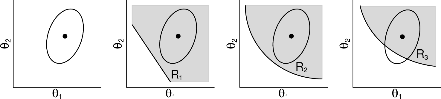
Consequently, a comparison region can be used for post hoc testing of the null hypothesis of interest. The logic of the approach is illustrated in figure 2. Comparison regions can be constructed very similarly to confidence regions. Consequently, confcomptwo supports drawing of both confidence regions and comparison regions.

Figure 2.

Presentation of a point estimate with a comparison region in a publication and three post hoc comparisons with regions of interest: The null hypotheses H ₀ : θ ∉ R ₁ and H ₀ : θ ∉ R ₂ can be rejected, and the null hypothesis H ₀ : θ ∉ R ₃ cannot be rejected. (This figure was previously published in Eckert and Vach [2020].)

1.3 Motivating examples

1.3.1 Diagnostic accuracy studies

Diagnostic accuracy is a genuine two-dimensional concept. By sharpening the criteria of a diagnostic test, one can reduce the number of false-positive (FP) decisions, but the number of true-positive (TP) decisions decreases, too. Consequently, the standard approach to analyzing the diagnostic accuracy of one test is to consider a pair of parameters such as sensitivity and specificity, positive and negative predictive values, the relative frequency of TP and FP decisions, or the positive and negative LRs. When one analyzes screening tests, it might also be of interest to relate sensitivity to the rate of positive test results because the aim is to achieve a high sensitivity while keeping the number of subjects to be followed up with as low as possible. When one compares two diagnostic tests, the focus is typically on the change in such a pair of parameter values.

There is no universal answer to the question of how to combine the two parameter estimates when a final decision about the usefulness of the test (or the new test in a comparative study) must be made (compare Vach, Gerke, and Hœilund-Carlsen [2012]). When one considers sensitivity and specificity, one is often advised to think about which parameter is more important in the specific clinical context. It is a rather straightforward idea to consider a weighted average of sensitivity and specificity. In practice, however, it seems cumbersome to agree on specific weights. The use of a range of weights has been considered with respect to analyzing sensitivity and specificity (Newcombe 2001) as well as when considering the rate of TP and FP decisions, particularly as part of a decision curve approach (Vickers 2008).

When different stakeholders post hoc perform analyses of a diagnostic accuracy study, each stakeholder may specify different weights and thresholds. Each stakeholder is interested in demonstrating that wθ ₁+(1−w) θ ₂ ≥ t for some w, t ∊ ℝ, that is, that the two parameters are within a certain half-space. If we want to satisfy all stakeholders, we have to reject the null hypothesis that the true parameters are outside the intersection of all of these half-spaces. This intersection is a convex subset of ℝ² and represents the common region of interest of all stakeholders.

1.3.2 Balancing between favorable and unfavorable consequences of an intervention

In evaluating a new intervention, one must often judge the balance between favorable and unfavorable consequences. Cost-effectiveness analyses are a classical example. Today, they are standard tools in health technology assessments and play important roles in deciding whether the additional costs can be justified by a gain in effectiveness or whether cost savings are so substantial that they can justify some loss in effectiveness. Similarly, there may be a need to balance the benefit and the risk associated with an intervention, and in benefit–risk assessments, it is common to consider a benefit–risk plane similar to a cost-effectiveness plane (Guo et al. 2010; Mt-Isa et al. 2014). Considering a two-dimensional approach can be particularly helpful to overcome some obstacles with noninferiority trials (Gladstone and Vach 2015).

In these types of analyses, because the parameters of interest are measured on differing scales, it is common to consider the ratio θ ₂/ θ ₁ for the joint evaluation of two parameter estimates and to define acceptable ratios r. Because θ ₂/ θ ₁ ≥ r is equivalent to θ ₂ − rθ ₁ ≥ 0, this still leads to linear hypotheses about the parameters of interest.

1.4 Construction of confidence regions and comparison regions

1.4.1 A general construction principle for comparison regions

Eckert and Vach (2020) describe the following general construction principle for a comparison region:

Lemma 1: Let φ_H denote a family of level-α tests for all half spaces H ⊂ Θ, that is, all subsets of the two-dimensional parameter space Θ of the type {( θ ₁, θ ₂)|w ₁ θ ₁+w ₂ θ ₂ ≥ t} for s ome w ₁, w ₂, t ∊ ℝ. φ_H provides a test for the null hypothesis H ₀ : θ ∊ H. Then (under some regularity conditions on the family of tests),

C : = \underset{ϕ H = 1}{\cap} \bar{H}

defines a level-α comparison region. Here $\bar{H}$ denotes the complement of a set H.

Roughly speaking, C can be interpreted as the intersection of all regions of interest that were “confirmed” by the tests. This general principle can be applied using the family of Wald tests or the family of LR tests. In both cases, the construction of comparison regions turns out to be very similar to the construction of confidence regions.

1.4.2 Explicit formulas for confidence regions and comparison regions

Given an estimate of the covariance matrix Σ of $\hat{θ}$ , applying the Wald test principle results in confidence and comparison regions of the type

C_{α} = {θ \in Θ ∣ {(θ - \hat{θ})}^{'} \hat{Σ}^{- 1} (θ - \hat{θ}) < c}

The only difference is the choice of the threshold c. $c = χ_{2, 1 - α}^{2}$ defines a (1 − α) confidence region. $c = χ_{1, 1 - 2 α}^{2}$ defines a level-α comparison region.

Using (asymptotic) LR tests as construction principles results in confidence and comparison regions of the type

C_{α} = {θ \in Θ ∣ l (θ) - l^{*} > - \frac{1}{2} c}

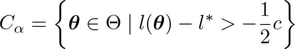
with l∗ denoting the value of the loglikehood function l(θ) at the maximum likelihood estimate. Again, the only difference is the choice of the threshold c. $c = χ_{2, 1 - α}^{2}$ defines a (1 − α) confidence region. $c = χ_{1, 1 - 2 α}^{2}$ defines a level-α comparison region for any α < 0.5.

Note that, for both approaches, it does hold that 74.2% confidence regions define 5% comparison regions. Consequently, 5% comparison regions are distinctly smaller than 95% confidence regions.

2 The confcomptwo command

2.1 The scope of confcomptwo

The command confcomptwo allows comparison and confidence regions to be drawn in two-parameter estimation problems. The approaches based on inverting Wald tests and on inverting LR tests are both supported. With the Wald-test-based approach, confcomptwo can be used as a postestimation command or as an immediate command specifying the five necessary input values. With the LR approach, the user must specify a program to compute a log likelihood depending on two parameters.

Eckert and Vach (2020) considered the case of a two-parameter likelihood, but the approach can also be applied to a two-parameter profile likelihood obtained by maximizing a higher-dimensional likelihood over the remaining nuisance parameters. Hence, confcomptwo also extends the pllf command to compute one-dimensional profile-likelihood-based confidence intervals. This command was provided by Royston (2007).

Actually, confcomptwo does not draw a line directly but uses a grid of points, plots the points, and connects the points with straight lines. The drawing is hence based on Stata’s twoway line command, but confcomptwo also supports representing the line with a series of small points. A comparison region and a confidence region can both be drawn simultaneously if both post hoc testing of hypotheses on half spaces and post hoc testing of single-point hypotheses are of interest. Furthermore, confcomptwo also allows following the recommendation of Eckert and Vach (2020) to draw comparison regions by a solid line and to draw confidence regions by a dotted line, reminding the user of the intended function—a comparison with a region of interest or with a single point.

2.2 The syntax of confcomptwo

The syntax of confcomptwo depends on whether you intend to use the Wald principle after fitting some model, the immediate form, or the LR principle.

If you intend to use confcomptwo as a postestimation command and apply the Wald test principle, the syntax is given by

confcomptwo parname1 parname2 [, confcomp_options twoway_options]

and the program expects to find entries with the column names parname1 and parname2 in the vector e(b), including the estimates and corresponding entries for the variances and covariance in the matrix e(V).

The immediate form has the syntax

confcomptwo #1 #2 , se1(real ) se2(real ) [corr(real ) confcomp_options twoway_options]

with #1 and #2 denoting the values of the two parameter estimates. The standard errors are provided using the required se1() and se2() options. The default correlation is corr(0).

If you intend to use the LR test principle, the syntax is given by

confcomptwo #1 #2 , call(expr ) [confcomp_options twoway_options linesearch_options]

and the expr in the required call() option describes the call of a user-written program that returns a log-likelihood value in r(ll). It should also return a binary indicator, r(inside), indicating whether the two arguments provided are within the allowed parameter values. The symbols #1 and #2 in this expression refer to the two parameter values at which the log likelihood should be evaluated. The parameter set allowed must be equal to R² or an open and convex subset of ℝ². The log-likelihood function must be strictly concave, and it must tend toward −∞ if the parameter values approach the boundary of the open set or if they tend toward ±∞.

confcomptwo allows the following confcomp_options:

alpha(real ) defines the level of the comparison region or 1 minus the level of the confidence region. The default is alpha(0.05).

points(numlist ) defines the points to be drawn. If numlist contains one number, it is interpreted as the number of points required. Otherwise, it defines a grid of directions in which the points are chosen relative to the parameter estimates. 0 and 1 refer to the direction “top of the graph”, 0.25 and 0.75 to the directions “right side of the graph” and “left side of the graph”, and 0.5 to the direction “bottom of the graph”. The default is points(101).

rescale(expr ) modifies the choice of the directions. The argument of the expression is noted with a # sign. Details are described in section 4.1.

loptsconf(line_options ) specifies the look of the line used to draw the confidence region. The default is loptsconf(lpat(dot)).

loptscomp(line_options ) specifies the look of the line used to draw the comparison region. The default is loptscomp(lpat(solid)).

mopts(marker_options ) specifies the look of the marker used to draw the point estimate. The default is mopts(mcol(black) msym(O)).

only(comp| conf) indicates that only confidence regions or comparison regions are to be computed.

nograph suppresses the graph.

savepoints(filename[, saveoptions]) saves the points computed as a Stata dataset with the given filename. The dataset includes the variables est1, est2, xi1, xi2, pcomp1, pcomp2, pconf1, and pconf2. The first two variables represent the input parameter values, and the next two variables represent the direction in which the point was searched for. The last four variables include the coordinates of the points used when drawing the lines. saveoptions can be any options allowed by Stata’s save command.

reverse exchanges the two axes in the plot. The default is to use the y axis for the first parameter and the x axis for the second parameter.

addplot(plot… [||plot…[…]][, below]) adds twoway plots to the graph and should work similarly to Stata’s addplot() option.

In addition, any twoway_options affecting the entire graph can be used except those involving a variable (such as the by() option). confcomptwo automatically generates a legend, and the label() suboption of the legend() option can be used to change the text. If the addplot() option is used, further entries are generated, and the order() suboption must be used to select the entries to be displayed.

If you are using the LR principle, you can also specify some linesearch_options, which are explained in section 4.3.

The dot line pattern style of Stata produces very small dots that are often hard to see. To address this issue, the options loptsconf() and loptscomp() also accept specifications of the following type:

points, n(integer ) [yxratio(real ) scatteroptions]

This indicates that the line is drawn by n() single points using the twoway scatter command. The points are drawn equidistantly, and their appearances can be changed using any option allowed with twoway scatter. yxratio() must be specified if the span of the y axis is not equal to the span of the x axis. If the savepoints() option is used, these additional points are also saved.

2.3 Stored results

confcomptwo stores in r(cmd) the command that was used to generate the graph. In combination with the savepoints() option, this allows the reproduction and further manipulation of the graph, if necessary. The point estimate is stored in the two scalars r(est1) and r(est2). If the Wald test principle is used, the variance–covariance matrix Σ is stored in the matrix r(Sigma).

2.4 Auxiliary commands to compute a log likelihood

To support the use of the LR principle, we provide the following three commands to compute the (profile) log likelihood for some standard situations that particularly appear in the context of analyzing diagnostic accuracy studies. All commands consider an open subset of R² as parameter space.

llproptwosamples #1 #2 [if] [in] [weight], var(varname) by(varname)

computes the log likelihood for a binary outcome variable with success probabilities differing between two subgroups. The log likelihood is evaluated for the two probabilities #1 and #2, referring to the two subgroups that must be labeled with the values 1 and 2. The following two options are required:

var(varname) defines the binary variable.

by(varname) defines the dichotomous grouping variable.

fweights are allowed; see [U] 11.1.6 weight. In particular, this likelihood can be used to evaluate sensitivity and specificity together (or positive and negative predictive values) for one diagnostic test. The parameter space is (0, 1)².

llproptwocats #1 #2 [if] [in] [weight], var(varname) cats(numlist)

computes the profile log likelihood for a categorical variable. The log likelihood is evaluated for the two probabilities #1 and #2, referring to the probabilities of two categories. The probabilities of the other categories remain unspecified. The following two options are required:

var(varname) defines the categorical variable.

cats(numlist) defines the two categories.

fweights are allowed; see [U] 11.1.6 weight. In particular, this likelihood can be used to evaluate the relative frequency of FP and TP decisions in analyzing one diagnostic test. The two arguments must be greater than 0, and their sum must be less than 1.

llriskcomptwosamples #1 #2 [if] [in] [weight], var(varlist) by(varname) {diff| logrr| logor| rr| or} [noisily maximize_options]

computes the profile log likelihood for two binary variables observed in two subgroups evaluated at two values #1 and #2, referring to the difference in the proportions between the two variables within subgroup 1 and within subgroup 2, respectively. The difference can be expressed as a difference, a log relative-risk, a log odds-ratio, a relative risk, or an odds ratio. The subgroups must be labeled with the values 1 and 2. The following options are required:

var(varlist) defines the two binary variables. The marginal proportion of the second variable is compared with the marginal proportion in the first variable when building differences, risk ratios, or odds ratios.

by(varname) defines the dichotomous grouping variable.

diff, logrr, logor, rr, or or specifies how the difference in proportions is expressed. Exactly one of these five options must be specified.

fweights are allowed; see [U] 11.1.6 weight. The noisily option allows inspection of the output of the ml max command, and the maximize_options are passed to this command. In particular, this specific likelihood can be used to evaluate changes in sensitivity and specificity in a comparative diagnostic accuracy study with a paired design. The parameter space depends on the choice of the option to express the difference.

NOTE: For relative risks and odds ratios, it typically makes little sense to consider weighted averages. However, confidence and comparison regions still provide a visual impression about the imprecision of the estimates.

All three commands also allow a force option that forces the computation of the log likelihood even if parameter values outside the parameter space are specified. This can be useful to plot regions for an estimate on the boundary. An example is given in section 3.5.

3 Examples

3.1 Example 1: Joint confidence region for two regression coefficients

Stata provides auto.dta, allowing study of the relation of mileage rating to the weight and the origin (foreign or domestic) of automobiles. The corresponding model is used in the Stata Base Reference Manual to illustrate linear regression. confcomptwo can supplement this standard analysis by depicting the joint uncertainty of the two regression coefficient estimates:

Figure 3.

A 95% confidence region for the two regression coefficients considered in example 1.

The resulting figure 3 informs us that the two regression coefficients are positively correlated. This is a simple consequence of the negative correlation between the two covariates: on average, foreign automobiles have lower weights than domestic automobiles.

Note that the parameter rescale was used in this example. This was necessary because the two estimates have very different magnitudes. The value 1,666 reflects the ratio between the span on the x axis (5) and the span on the y axis (0.003). Here we also followed the tradition of drawing confidence regions with solid lines.

3.2 Example 2: Analysis of a single-arm diagnostic accuracy study

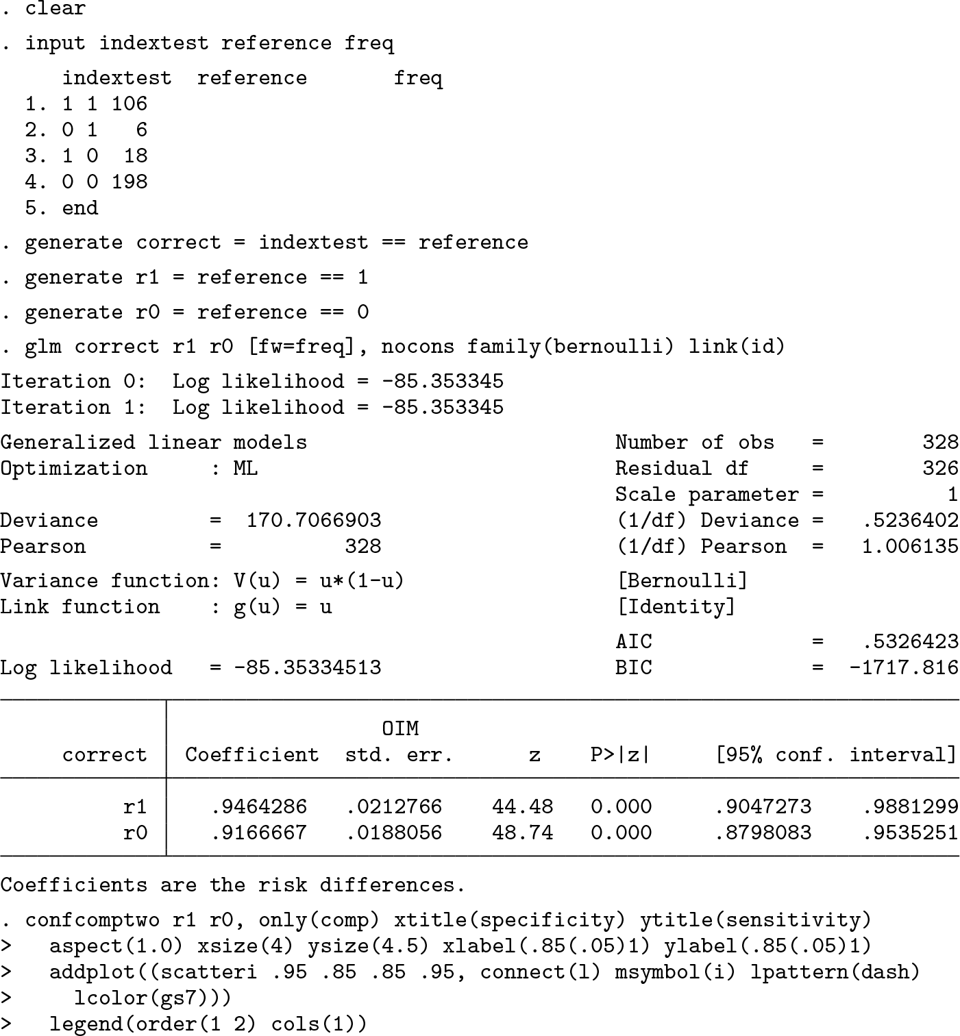
Xu et al. (2017) presented a study on the diagnosis of hemodynamically significant coronary stenosis defined by fractional flow reserve ≤ 0.80. One goal was to assess the diagnostic accuracy of angiography-based quantitative flow ratio measurements using the same cutpoint. Using fractional flow reserve as the reference standard, they observed a sensitivity of 106/112 = 94.6% and a specificity of 198/216 = 91.7% based on overall 328 interrogated vessels.

Computing the standard errors of sensitivity and specificity manually, we can use the immediate version of confcomptwo to obtain a two-dimensional Wald-test-based comparison region:

To facilitate the interpretation of the comparison region, we can add a reference line referring to an average of sensitivity and specificity of 0.9 to mimic a specific posttest situation:

Figure 4.

Wald-test-based 5% comparison region for sensitivity and specificity in example 2 with a reference line added

The resulting figure 4 allows the comparison of the reference line with the comparison region. The line is located below the comparison region. This supports the conclusion that the average between sensitivity and specificity is above 0.9.

In the computations carried out above, we have taken advantage of the fact that sensitivity and specificity are based on two separate samples, and we therefore know that they are uncorrelated when conditioning on the observed sample sizes. If manual computation of standard errors is to be avoided, we can use the postestimation version of confcomptwo. This requires obtaining the estimates of sensitivity and specificity together from one command and simultaneously an estimate of the variance–covariance matrix. One can approach this by generating a dataset with the study results, translating the index test results into a variable correct indicating correct test results, and modeling this variable in a generalized linear model with identity-link and Bernoullitype variances as a function of the results of the reference test encoded by two indicator variables:

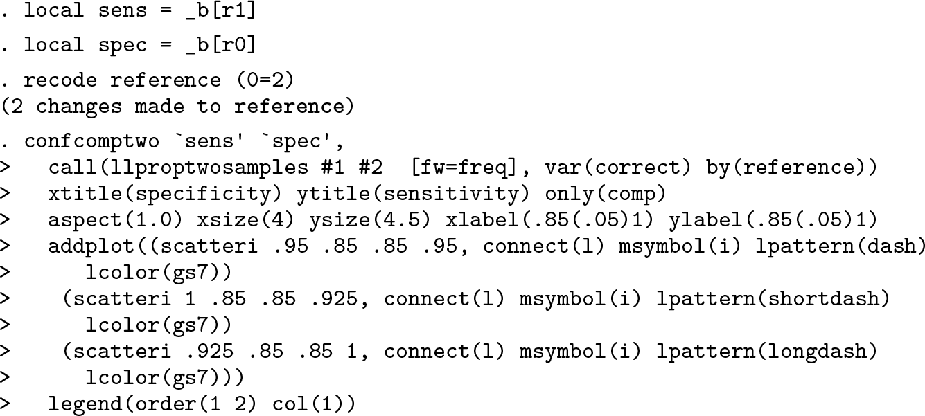
To obtain LR-test-based regions, we use the llproptwosamples command because sensitivity and specificity are proportions from two independent samples. To do so, we must store the values of sensitivity and specificity and recode the variable reference because llproptwosamples expects the two groups to be labeled with the values 1 and 2:

Figure 5.

LR-test-based 5% comparison regions for sensitivity and specificity in example 2 with three reference lines added

The resulting figure 5 indicates that the shape of the LR-test-based region is distinctly different from the shape of the Wald-test-based region. This can be explained by the proximities of sensitivity and specificity to 1.0. Two further reference lines were added to the figure, giving the sensitivity twice the weight of specificity and vice versa. For all three choices of weights, one can conclude that the weighted average of sensitivity and specificity is above 0.9.

3.3 Example 3: Analysis of a paired diagnostic accuracy study

Ng et al. (2008) reported a study comparing the diagnostic accuracy of ¹⁸F-fluoro-2-deoxyglucose positron emission tomography with extended-field multidetector computed tomography for the detection of distant malignancies in patients with oropharyngeal or hypopharyngeal squamous cell carcinoma. All patients were followed up with for at least 12 months or until death to construct a reference standard. For a suspected malignant lesion, a biopsy of the tissue was taken if possible or close clinical and imaging followup was performed. Distant malignancies were found in 26 out of 160 patients enrolled in the study. The two diagnostic tools investigated yielded a sensitivity/specificity of 50.0%/97.8% and of 76.9%/94.0%. The study was conducted in a paired design, so the results can be summarized in a 2 × 2 × 2 contingency table with the frequencies for each combination of results for the two index tests to be compared and the reference standard. This contingency table is available in studyng.dta.

In a first analysis, the interest is in studying the changes in sensitivity and specificity when replacing test 1 with test 2. Because there are no simple formulas to compute the standard errors of the change, we use the postestimation version of confcomptwo to compute Wald-test-based regions. This requires the derivation of the estimates and their covariance matrices with one estimation command. We hence compute estimates of the sensitivities and specificities of both tests—that is, simple relative frequencies—by fitting four intercept-only generalized linear models with identity-link and Bernoullitype variances, saving the estimates, using Stata’s suest to obtain the joint covariance matrix, and finally using the nlcom command to obtain the two differences of interest and their covariance matrices. In this setting, it might be of interest to also test the null hypotheses of no change in both sensitivity and specificity. Consequently, both comparison and confidence regions are drawn.

Figure 6.

Wald-test-based 5% comparison and 95% confidence regions for the changes in sensitivity and specificity in example 3 with three reference lines added

The resulting figure 6 indicates a distinct improvement in sensitivity and a slight deterioration in specificity. Because of the low prevalence of the disease state of interest, the precision of the estimate of the change in sensitivity is rather low. We included three lines in the graph referring to the situation where some weighted averages of the changes in sensitivity and specificity are equal to zero. The dotted line refers to equal weights, and we can conclude that the increase in sensitivity is larger than the loss in specificity. However, because the sensitivity of the standard test is rather low and the specificity is already rather high, we are actually interested in a substantial improvement in sensitivity. The line with short dashes refers to giving the change in sensitivity a weight 1.5 times higher than the weight given to the change in specificity, and the line with long dashes refers to weighting the change in sensitivity two times higher than the change in specificity. In all three cases, the line does not hit the comparison region. Consequently, we can conclude that the gain in sensitivity is at least twice as great as the loss in specificity.

Note the use of the aspect() and yxratio() options. Because the precision of the change in sensitivity is much lower than the precision of the change in specificity, the span of the y axis is 0.6, whereas the span of the x axis is only 0.3. The option aspect(2) ensures that a change of 0.1 is nevertheless represented by the same distance in y and x direction in the visual inspection of the graph. The option yxratio(2) ensures that the points drawn to represent the confidence interval are equidistant.

To obtain LR-test-based regions, we store the two estimates, and then we use the llriskcomptwosamples command. The latter requires recoding the reference variable:

The resulting figure is not shown, because it is nearly identical to the one obtained using the Wald test.

Next we present a second analysis considering the change in the relative frequency of TP and FP decisions. Wald-test-based comparison and confidence regions can be approached similarly to above, starting with the empirical estimates of the four relative frequencies expressed as estimates from an intercept-only generalized linear model:

Figure 7.

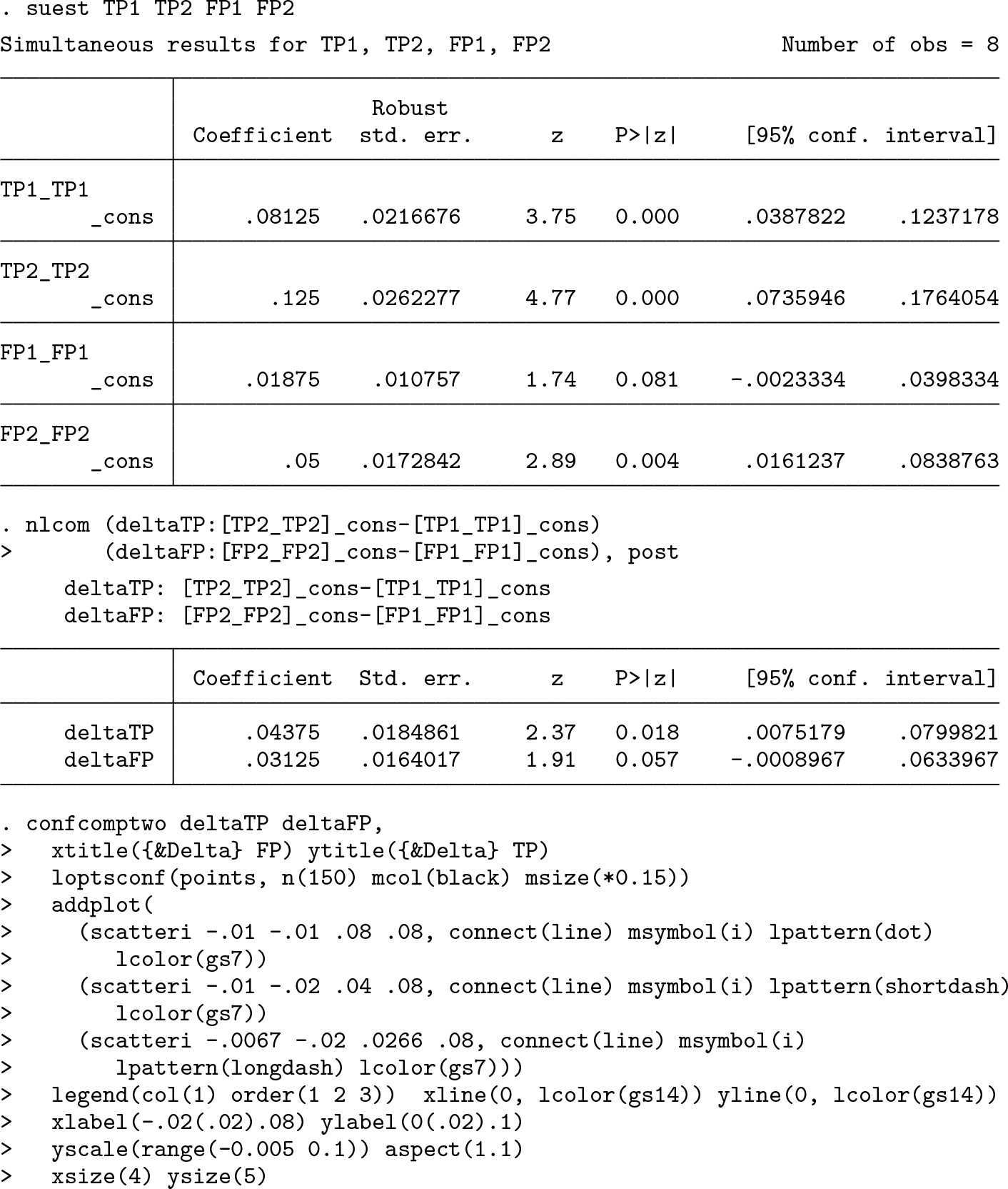
Wald-test-based 5% comparison and 95% confidence regions for the change in the relative frequency of TP and FP decisions in example 3 with three reference lines added

In the resulting figure 7, we observe an increase in the frequency of TP decisions by 4.4%, which is about a factor 1.5 higher than the increase in FP decisions. This looks less impressive than the changes in sensitivity and specificity, which are due to the low prevalence of the disease state of interest in this example. Different stakeholders may have different views on how many additional FP decisions they may accept for one additional TP decision. If they maximally accept only one FP, they are interested in demonstrating that the difference between the TP rate and the FP rate is above 0, that is, in points above the dotted line referring to the weights 1 and −1 for the TP rate and the FP rate, respectively. If they are willing to accept two FP decisions for a gain in one TP decision, they are interested in points above the line with short dashes referring to the weights 1 and −2 for the TP rate and the FP rate, respectively. If they are willing to accept three FP decisions for a gain in one TP decision, they are interested in points above the line with long dashes, which refers to the weights 1 and −3 for the TP rate and the FP rate, respectively. We can observe that they can conclude that the new test implies an advantage only in the last case.

To use the LR approach, we must write a specific program to evaluate the log likelihood. We will present this in section 5 after we have taken a closer look at the formulas used by llriskcomptwosamples.

3.4 Example 4: Joint evaluation of benefit and risk in a randomized controlled trial

Saxer et al. (2018) reported the results of a randomized controlled trial comparing two surgical techniques to be used to treat femoral neck fractures in patients over 60 years of age requiring hemiarthroplasty. The aim was to demonstrate that an anterior minimally invasive approach is beneficial to patients in terms of accelerated remobilization compared with a standard lateral Hardinge approach. The primary endpoint was early mobility evaluated at three weeks via the “timed up and go” (TUG) test. This test measures the time needed to get up from a chair, to walk a distance of three meters, and to sit down again. A 20% reduction was regarded as clinically relevant. Various secondary endpoints were considered. We focus here on the endpoint occurrence of local infections, reflecting a potential safety concern about the minimally invasive approach.

The study analyzed the primary endpoint by applying a regression model with the covariates treatment arm, age, and functional independence measure at baseline to the log-transformed TUG values. The back-transformed treatment effect was interpreted as an estimate of the median reduction in time required for the TUG. This resulted in an effect estimate corresponding to a 21.5% reduction. The frequency for local infections was 5 out of 96 in the lateral Hardinge arm and 7 out of 79 in the anterior minimally invasive arm, corresponding to an increase of 3.6 infections in 100 patients.

confcomptwo can be used to visualize the joint uncertainty in these two estimates in a benefit–risk plane. One can approach this by computing the two estimates using regression commands, combining these results using the suest command to determine the correlation, and finally using confcomptwo as a postestimation command:

Figure 8.

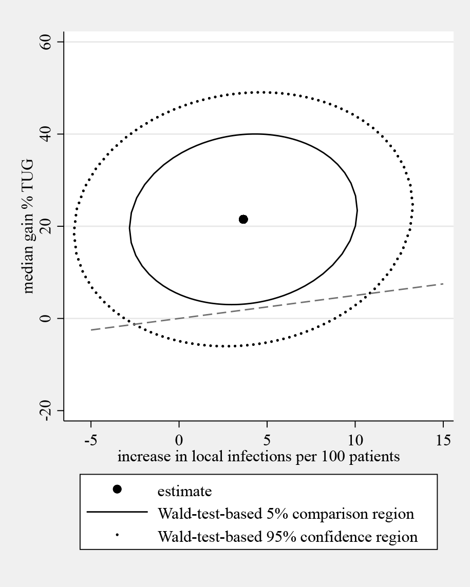
Wald-test-based 5% comparison and 95% confidence regions for the gain in TUG and the increase in number of local infections in example 4

The resulting figure 8 indicates that it is hard to draw firm conclusions because of the substantial imprecision of the estimates. Only if we would regard a very small gain in TUG time as justification for an increase by 1 local infection in 100 patients could we conclude that the true parameter values are above this line. To illustrate this, we show a reference line referring to a ratio between the gain in TUG and the number of additional local infections per 100 patients of 0.5. For 10 additional local infections, this would imply a 5% gain in TUG.

3.5 Example 5: LR-test-based regions for an estimate on the boundary

If the parameter space of a two-dimensional parameter estimation problem is bounded, it is possible for the point estimate to be on the boundary. LR-test-based comparison and confidence regions are then still defined, but drawing is slightly more complicated. However, if we restrict the drawing to directions into the inner part of the parameter space, it is still possible to draw regions. This is illustrated by an artificial example from a single-arm diagnostic study with a sensitivity estimate of 1.0, which results in figure 9:

Figure 9.

LR-test-based 5% comparison region for sensitivity and specificity in example 5

Note that it was necessary to use the force option to ensure that the log likelihood could be evaluated at the point estimate, and note that the points() option was used to explicitly specify the range of directions to be considered.

4 Methods and formulas

4.1 Parameterization of directions

The following two subsections describe how to determine the point on the boundary of a comparison or confidence region when looking from the point estimate in a certain direction ξ ∊ ℝ²\(0, 0). A first, straightforward choice for the directions may be ξ_t = (cos t, sin t)′ with values t from the grid t_j = {(j − 1)/(J − 1)}2π for j = 1,…, J with J denoting the overall number of directions considered. This implies that all angles between two neighboring directions are equal, and this is indeed also the default choice in confcomptwo. However, the equality of angles holds only with respect to the parameter space with the Euclidean metric. It does not hold with respect to the plane in which we plot the regions in the figure we want to create, because the two dimensions are typically rescaled as part of the drawing process. Moreover, equal angles are optimal only if the shape of the region is close to a circle, and it can be a poor choice in the case of other shapes. Hence, confcomptwo also offers a more general approach: A list of values t_j can be provided (using the points() option with a numlist), and a function s(t) can be provided in the rescale() option. The directions are determined as ξ_t = {s(t) cos t, sin t}′. If s(t) is chosen as a constant, this just implies a rescaling of the directions with respect to the parameter shown on the y axis.

If the units of the axes in the plot plane roughly correspond to the same physical length and the shape of the regions is close to a circle, the default value of J = 101 is typically large enough to ensure that the boundary lines of the comparison and confidence regions appear as smooth lines when plotting the calculated points in a graph and connecting them with straight lines.

4.2 Drawing comparison and confidence regions based on the Wald test principle

Given a direction ξ ∊ ℝ²\(0, 0), the point on the boundary of C_α in this direction (starting at $\hat{θ}$ ) is given by

θ (ξ) = \hat{θ} + \hat{Σ} ξ \sqrt{\frac{χ_{1, 1 - 2 α}^{2}}{ξ^{'} \hat{Σ} ξ}}

(When $ξ^{'} \hat{Σ} ξ$ equals 0, we set θ ( ξ ) = $\hat{θ}$ .) C_α can easily be drawn by plotting and connecting the points θ ( ξ _t ) with t chosen as described in the previous subsection.

When we use the Wald test principle to construct (1 − α) confidence regions for θ , the points are given by

θ (ξ) = \hat{θ} + \hat{Σ} ξ \sqrt{\frac{χ_{2, 1 - α}^{2}}{ξ^{'} \hat{Σ} ξ}}

4.3 Drawing comparison and confidence regions based on the LR test principle

Given a direction ξ ∊ ℝ²\(0, 0), the point on the boundary of C_α in this direction [starting at $\hat{θ}$ _ML with the log-likelihood value l∗ = l( $\hat{θ}$ _ML)] can be determined by solving the equation

l ({\hat{θ}}_{ML} + γ ξ) = l^{*} - \frac{1}{2} χ_{1, 1 - 2 α}^{2}

for γ > 0. Because γ ↦ l( $\hat{θ}$ _ML + γξ) is a strictly monotone decreasing function with maximum 0, the solution γ( ξ ) is unique and can easily be determined by a simple line search. We can then plot all points $\hat{θ}$ _ML + γ( ξ _t ) ξ _t with t chosen as described above and connect these points.

The same approach has been recently recommended by Jaeger (2016) for plotting LR-test-based confidence regions. This requires just the replacement of $χ_{1, 1 - 2 α}^{2}$ with $χ_{2, 1 - α}^{2}$ .

The line search is conducted as follows. Let el(γ) := l( $\hat{θ}$ _ML + γξ) and τ := l∗ − $(1 / 2) χ_{1, 1 - 2 α}^{2}$ . When the point $\hat{θ}$ _ML + γξ _t is outside the parameter space Θ of interest (as indicated by the returned value of r(inside)), $\tilde{l} (γ)$ is set to −∞. For a starting value γ ₀ > 0, we check whether $\tilde{l} (γ)$ is less than, greater than, or equal to τ. In the first case, we decrease γ by the factor 1/f until $\tilde{l} (γ)$ is greater or equal to τ. In the second case, we increase γ by the factor f until $\tilde{l} (γ)$ is less than τ. The last two values in this sequence are then used as starting values for a bisectioning search, making use of the regula falsi. The bisectioning stops if the absolute value of the difference between $\tilde{l} (γ)$ and τ is less than 10⁻⁴, a value that can be changed by the lstoler() option.

For the first grid value t, γ ₀ is specified by the lsstartgamma() option with a default value of 1.0, and f is specified by the lsstartfactor() option with a default value of 10.0. For subsequent grid values, γ ₀ is chosen as the final value from the previous search, and f is specified by the lsfactor() option with a default value of 1.02 in the case of 100 or more points and is linearly increasing up to 2.0 in the case of only 2 points. These choices usually work properly if the number of points J is large enough. You can use the lstrace() option to obtain information about the γ values and corresponding points and log-likelihood values considered in each line search. It is well known that the regula falsi is a suboptimal procedure to determine the root of a concave function. However, using a factor of 1.02 in the line search implies that usually only one bisectioning step is required; hence, there is no need to consider more efficient algorithms. The use of the optimal γ value of the previous step as the starting point for the line search implies that usually only one or two line search steps are required before starting bisectioning.

When the call to the program provided by the user results in an error code different from 0 or the log likelihood evaluates to a missing value, no point is plotted in the corresponding direction, and a warning message is shown.

The validity of the comparison and confidence regions drawn depends heavily on the correct specification of the values of the maximum likelihood (ML) estimate. Hence, confcomptwo automatically performs two checks. First, every log-likelihood value computed is compared with the value obtained for the specified ML estimate, and the program stops with an error message if the difference is larger than 10⁻⁵. Second, after constructing a point on the boundary, the log likelihood is also evaluated at the parameter value obtained by moving only 0.01% into the direction of the point.

4.4 The llproptwosamples command

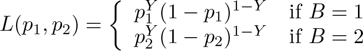
The llproptwosamples command refers to the following likelihood for a single observation of the binary variable Y and the grouping variable B:

L (p_{1}, p_{2}) = {\begin{array}{l} p_{1}^{Y} {(1 - p_{1})}^{1 - Y} & if B = 1 \\ p_{2}^{Y} {(1 - p_{2})}^{1 - Y} & if B = 2 \end{array}

The command computes the sum of logL(p ₁, p ₂) over all observations.

4.5 The llproptwocats command

The llproptwocats command refers to the following likelihood for a single observation of the categorical variable Y with prespecified categories c ₁ and c ₂:

L (p_{1}, p_{2}) = {\begin{array}{l} p_{1} & if Y = c_{1} \\ p_{2} & if Y = c_{2} \\ 1 - p_{1} - p_{2} & otherwise \end{array}

The command computes the sum of logL(p ₁, p ₂) over all observations.

4.6 The llriskcomptwosamples command

The implementation of the llriskcomptwosamples command requires one to find a parameterization for the joint distribution of two binary variables Y ₁ and Y ₂, which allows one to fix the difference (risk ratio, odds ratio, log risk-ratio, log odds-ratio) between the two marginal probabilities while allowing the other parameters to vary freely without any further restrictions. We use a tetrachoric parameterization (Pearson 1900), which is simple to implement in Stata because of the availability of the binormal() function, allowing the computation of the joint cumulative distribution of a bivariate normal distribution with correlation ρ, marginal means 0, and marginal variances 1. This parameterization assumes that Y ₁ and Y ₂ are derived from two continuous random variables Z ₁ and Z ₂ following such a bivariate normal distribution by dichotomization at q_k = Φ⁻¹(p_k) for k = 1, 2, with p_k denoting the prevalence of Y_k. The likelihood of an observation (Y ₁, Y ₂) is then given by

\begin{matrix} L^{Y_{1}} {​^{= 1, Y_{2}}}^{= 1} (p_{1}, p_{2}, ρ) & = P (Z_{1} < q_{1}, Z_{2} < q_{2}) = b i n o r m a l (q_{1}, q_{2}, ρ) \\ L^{Y_{1}} {​^{= 1, Y_{2}}}^{= 0} (p_{1}, p_{2}, ρ) & = P (Z_{1} < q_{1}, Z_{2} > q_{2}) = P (Z_{1} < q_{1}) - P (Z_{1} < q_{1}, Z_{2} < q_{2}) \\ ​ & = p_{1} - b i n o r m a l (q_{1}, q_{2}, ρ) \\ L^{Y_{1}} {​^{= 1, Y_{2}}}^{= 1} (p_{1}, p_{2}, ρ) & = P (Z_{1} > q_{1}, Z_{2} < q_{2}) = P (Z_{2} < q_{2}) - P (Z_{1} < q_{1}, Z_{2} < q_{2}) \\ ​ & = p_{2} - b i n o r m a l (q_{1}, q_{2}, ρ) \\ L^{Y_{1}} {​^{= 1, Y_{2}}}^{= 0} (p_{1}, p_{2}, ρ) & = P (Z_{1} > q_{1}, Z_{2} > q_{2}) \\ ​ & = 1 - P (Z_{1} < q_{1}) - P (Z_{2} < q_{2}) + b i n o r m a l (q_{1}, q_{2}, ρ) \\ ​ & = 1 - p_{1} - p_{2} + b i n o r m a l (q_{1}, q_{2}, ρ) \end{matrix}

With B denoting the grouping variable, the profile log likelihood is then obtained by maximizing for b = 1, 2

\sum_{i, B_{i} = b} \log L^{y_{1 i}, y_{2 i}} (ρ^{b}, p_{1}^{b}, p_{2}^{b})

under the constraints on p ₁ ^b and p ₂ ^b specified when calling the command and then summing up the two values.

The maximization task is approached using Stata’s ml command. The correlation ρ is expressed as tanh ρ′ with ρ′ varying between −∞ and +∞ and p ₁ and p ₂ are expressed as functions of the given value ζ of the constraint in the group considered (and the type of the constraint) and a freely varying parameter α as follows:

Consequently, the profile log likelihood is obtained by maximizing

\sum_{b = 1, 2} \sum_{i, B_{i} = b} \log {\tilde{L}}^{y_{1 i}, y_{2 i}} (ρ_{b}^{'}, α_{b}, ζ_{b})

with

{\tilde{L}}^{y_{1}, y_{2}} (ρ^{'}, α, ζ) = L^{y_{1}, y_{2}} {\tanh ρ^{'}, p_{1} (α, ζ), p_{2} (α, ζ)}

over ρ ₁′, ρ ₂′, α ₁, and α ₂.

Note that the profile likelihood can be interpreted as a conditional likelihood given the frequencies of B = 1 and B = 2 as well as an unconditional likelihood because, in the latter case, the additional contribution depending on the prevalence π does not affect the maximization task.

5 An example involving a user-defined program to compute the profile log likelihood

To continue with example 3 in section 3.3, we need an appropriate parameterization of the joint distribution of Y ₁, Y ₂, and D. We use the fact that the change in relative frequency of TP decisions Δ_TP can be related to the change in sensitivity Δ_sens and the prevalence π, and the change in relative frequency of FP decisions Δ_FP can be related to the change in specificity Δ_spec and the prevalence. To be precise, we have Δ_sens = Δ_TP/π and Δ_spec = −Δ_FP/(1 − π). We now use the framework developed for the llriskcomptwosamples command in section 4.6 in the case of using the diff option. With the notation introduced there, we can express the log likelihood for a trivariate observation (Y ₁, Y ₂, D) as

\begin{array}{l} \log {\tilde{L}}^{Y_{1}, Y_{2}} {ρ_{0}^{'}, α_{0}, - Δ_{FP} / (1 - π)} + \log (1 - π) & if D = 0 \\ \log {\tilde{L}}^{Y_{1}, Y_{2}} (ρ_{1}^{'}, α_{1}, Δ_{TP} / π) + \log π & if D = 1 \end{array}

The profile log likelihood for given values of Δ_TP and Δ_FP is then obtained by maximization over $ρ_{0}^{'}, ρ_{1}^{'}$ , α ₀, α ₁, and logit π.

To apply the LR approach, we must provide a program to compute the profile loglikelihood function. We start with defining the program tetrall to define the log likelihood corresponding to a tetrachoric parameterization of a bivariate binary distribution. We then define the program modeldeltaFPTP to compute the log likelihood suitably for Stata’s ml command, and we finally define the program lldeltaFPTP to compute the profile log likelihood by calling ml.

Figure 10.

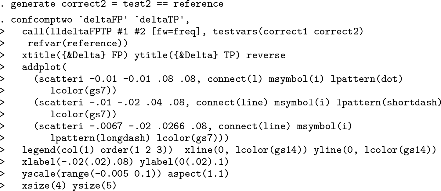
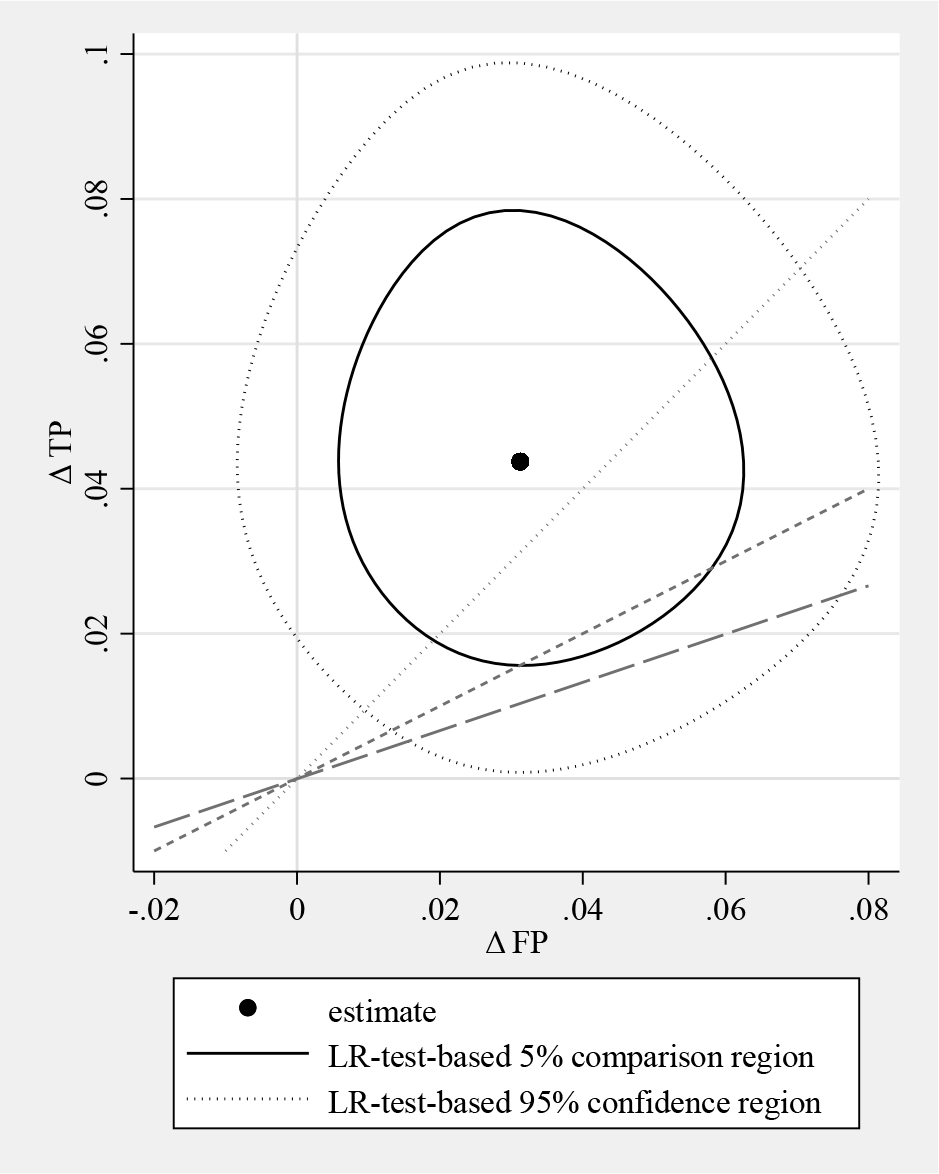
LR-test-based 5% comparison and 95% confidence regions for the change in the relative frequency of FP and TP decisions in example 3

In the resulting figure 10, we can observe that the shape of the regions based on the LR test principle deviates distinctly from the elliptic shape of the Wald-test-based regions. However, the conclusions remain the same.

6 Conclusions

In some areas of statistical applications (such as diagnostic accuracy studies), it is essential to present a joint evaluation of two parameter estimates. Two-dimensional confidence and comparison regions are useful tools supporting this goal. Drawing such regions is quite challenging and not easily accomplished within the existing graphical tools in Stata. Therefore, the confcomptwo command presented in this article can be seen as a useful and necessary addition that may stimulate an improved presentation of estimation results in specific settings.

The examples presented in this article indicate that Wald-test-based and LR-test-based comparison regions may substantially differ in their shape. First investigations of finite-sample properties (Eckert and Vach 2020) suggest that LR-test-based comparison regions are closer to their nominal level than Wald-test-based comparison regions. Therefore, we recommend using LR-test-based comparison regions. However, LR-test-based comparison regions also rely on inverting tests that are only asymptotically valid. In the long run, the use of exact methods might be desirable.

The optimal choice of directions for drawing the boundary points of the regions is a nontrivial problem. confcomptwo gives the user a flexible framework for the choice of directions, but in principle this choice can be optimized automatically. This holds at least in the case of Wald-test-based regions, for which the shape is determined by the variance–covariance matrix.

It can be seen as a disadvantage of confcomptwo that the computation of the ML estimates is decoupled from the drawing of the LR-test-based confidence regions. However, it is not trivial to derive profile likelihood functions from ordinary likelihood functions when nonstandard transformations of the parameters (such as those considered in our examples) are involved.

8 Programs and supplemental materials

Supplemental Material, sj-zip-1-stj-10.1177_1536867X231175314 - Visualizing uncertainty in a two-dimensional estimate using confidence and comparison regions

Supplemental Material, sj-zip-1-stj-10.1177_1536867X231175314 for Visualizing uncertainty in a two-dimensional estimate using confidence and comparison regions by Maren Eckert and Werner Vach in The Stata Journal

Footnotes

7 Acknowledgment

This work was supported by the German Research Foundation (DFG) [VA 88/5-1].

8 Programs and supplemental materials

To install a snapshot of the corresponding software files as they existed at the time of publication of this article, type

References

Eckert

Vach

2020. On the use of comparison regions in visualizing stochastic uncertainty in some two-parameter estimation problems. Biometrical Journal 62: 598–609. https://doi.org/10.1002/bimj.201800232.

Gladstone

B. P.

Vach

2015. Analyzing noninferiority trials: It is time for advantage deficit assessment—An observational study of published noninferiority trials. Open Access Journal of Clinical Trials 7: 11–21. https://doi.org/10.2147/OAJCT.S74821.

Guo

J. J.

Pandey

Doyle

Bian

Lis

Raisch

D. W.

2010. A review of quantitative risk-benefit methodologies for assessing drug safety and efficacy-report of the ISPOR risk-benefit management working group. Value in Health 13: 657–666. https://doi.org/10.1111/j.1524-4733.2010.00725.x.

Jaeger

2016. Computation of two- and three-dimensional confidence regions with the likelihood ratio. American Statistician 70: 395–398. https://doi.org/10.1080/00031305.2016.1182946.

Mt-Isa

Hallgreen

C. E.

Wang

Callréus

Genov

Hirsch

, et al. 2014. Balancing benefit and risk of medicines: A systematic review and classification of available methodologies. Pharmacoepidemiology and Drug Safety 23: 667–678. https://doi.org/10.1002/pds.3636.

Newcombe

R. G.

2001. Simultaneous comparison of sensitivity and specificity of two tests in the paired design: A straightforward graphical approach. Statistics in Medicine 20: 907–915. https://doi.org/10.1002/sim.906.

S.-H.

Chan

S.-C.

Liao

C.-T.

Chang

J. T.-C.

S.-F.

Wang

H.-M.

Chin

S.-C.

Lin

C.- Y.

Huang

S.-F.

Yen

T.-C.

2008. Distant metastases and synchronous second primary tumors in patients with newly diagnosed oropharyngeal and hypopharyngeal carcinomas: Evaluation of ¹⁸F-FDG PET and extended-field multi-detector row CT. Neuroradiology 50: 969–979. https://doi.org/10.1007/s00234-008-0426-2.

Pearson

1900. Mathematical contributions to the theory of evolution. VII: on the correlation of characters not quantitatively measurable. Philosophical Transactions of the Royal Society of London, Series A 195: 1–47. https://doi.org/10.1098/rsta.1900.0022.

Royston

2007. Profile likelihood for estimation and confidence intervals. Stata Journal 7: 376–387. https://doi.org/10.1177/1536867X0700700305.

10.

Saxer

Studer

Jakob

Suhm

Rosenthal

Dell-Kuster

Vach

Bless

2018. Minimally invasive anterior muscle-sparing versus a transgluteal approach for hemiarthroplasty in femoral neck fractures—A prospective randomised controlled trial including 190 elderly patients. BMC Geriatrics 18: 222. https://doi.org/10.1186/s12877-018-0898-9.

11.

Vach

Gerke

Hœilund-Carlsen

P. F.

2012. Three principles to define the success of a diagnostic study could be identified. Journal of Clinical Epidemiology 65: 293–300. https://doi.org/10.1016/j.jclinepi.2011.07.004.

12.

Vickers

A. J.

2008. Decision analysis for the evaluation of diagnostic tests, prediction models, and molecular markers. American Statistician 62: 314–320. https://doi.org/10.1198/000313008x370302.

13.

Qiao

Chen

Yang

Guo

, et al. 2017. Diagnostic accuracy of angiography-based quantitative flow ratio measurements for online assessment of coronary stenosis. Journal of the American College of Cardiology 70: 3077–3087. https://doi.org/10.1016/j.jacc.2017.10.035.

Supplementary Material

Please find the following supplemental material available below.

For Open Access articles published under a Creative Commons License, all supplemental material carries the same license as the article it is associated with.

For non-Open Access articles published, all supplemental material carries a non-exclusive license, and permission requests for re-use of supplemental material or any part of supplemental material shall be sent directly to the copyright owner as specified in the copyright notice associated with the article.

0.01 MB

0.00 MB