Sage Journals: Discover world-class research

Abstract

In this article, we introduce the xtgrangert command, which implements the panel Granger noncausality testing approach developed by Juodis, Karavias, and Sarafidis (2021, Empirical Economics 60: 93–112). This test offers superior size and power performance to existing tests, which stem from the use of a pooled estimator that has a faster $\sqrt{N T}$ convergence rate. The test has several other useful properties: it can be used in multivariate systems; it has power against both homogeneous and heterogeneous alternatives; and it allows for cross-section dependence and cross-section heteroskedasticity.

Keywords

st0706 xtgrangert xtgrangert postestimation panel data Granger causality Nickell bias heterogeneous panels half-panel jackknife cross-section dependence

1 Introduction

Predictive (Granger) causality and feedback is an important aspect of applied time-series and longitudinal panel-data analysis. Granger (1969) developed a statistical concept of causality between two or more time-series variables, according to which a variable x “Granger-causes” a variable y if the variable y can be better predicted using past values of both x and y rather than using solely past values of y. The concept of “Granger causality” has been widely adopted in economics, medicine, chemistry, physics, biology, engineering, and beyond.

Granger causality is also useful when the data consist of multiple time series, as in the case of panel data. Methods on testing for Granger causality using panel-data models are very well cited and widely available in standard econometric software. Prominent examples include the generalized method of moments (GMM) approach of Holtz-Eakin, Newey, and Rosen (1988), which is valid for homogeneous panels with a few time-series observations (T), and the methods of Dumitrescu and Hurlin (2012) and Emirmahmutoglu and Kose (2011), suitable for heterogeneous, large-T panels. The GMM approach of Holtz-Eakin, Newey, and Rosen (1988) has been implemented in Stata by Abrigo and Love (2016) with the command pvargranger, whereas the method of Dumitrescu and Hurlin (2012) is available in both EViews and Stata; see, for example, the command xtgcause by Lopez and Weber (2017).

Recently, Juodis, Karavias, and Sarafidis (2021) developed a new method for testing the null hypothesis of no Granger causality, which is valid in models with homogeneous or heterogeneous coefficients. The novelty of their approach lies in the fact that under the null hypothesis, the Granger-causality parameters equal zero, and thus they are homogeneous. This allows the use of a pooled fixed effects-type estimator for these parameters only, which guarantees a $\sqrt{N T}$ convergence rate, where N denotes the number of cross-sectional units in the panel and T denotes the number of time-series observations in the panel.¹ To account for the so-called Nickell bias of the pooled estimator, their testing procedure makes use of the half-panel jackknife (HPJ) method of Dhaene and Jochmans (2015). The resulting approach works very well under circumstances that are empirically relevant: many cross-section units, a moderate time dimension, heterogeneous nuisance parameters, and high persistence.

The method of Juodis, Karavias, and Sarafidis (2021) has a number of advantages relative to existing approaches. In particular, the GMM approach of Holtz-Eakin, Newey, and Rosen (1988) is not appealing when T is (even moderately) large. This is due to the well-known problem of using too many instruments, which often renders the usual GMM-based inference highly inaccurate; see, for example, Bun and Sarafidis (2015) and remark 8 in Juodis and Sarafidis (2022). Moreover, when feedback based on past own values is heterogeneous (that is, the autoregressive parameters vary across individuals), inferences may not be valid even asymptotically. On the other hand, while the method of Dumitrescu and Hurlin (2012) accommodates heterogeneous slopes under both null and alternative hypotheses, their test statistic is theoretically justified only for sequences where N/T ² → 0. This implies that when T is sufficiently smaller than N, that is, T << N, this method can suffer from substantial size distortions. In an extended Monte Carlo experiment, Juodis, Karavias, and Sarafidis (2021) show that their method outperforms the method of Dumitrescu and Hurlin (2012) in terms of power.

The present article introduces a new command, xtgrangert, that implements the Granger noncausality test of Juodis, Karavias, and Sarafidis (2021). The command reports the Wald test statistic and its p-value, the null and the alternative hypotheses, and regression results with respect to the HPJ bias-corrected pooled estimator. The command offers options for both manual and automatic lag-length selection, using a Bayesian information criterion (BIC). The command further allows for cross-sectional dependence and cross-sectional heteroskedasticity in the errors. Finally, the command can test for Granger causality in equations with multiple relevant variables.² The panel must be balanced.

Notably, by construction xtgrangert is computationally faster than xtgcause, especially so when N is relatively large. This is because the former is based on a single, pooled regression, whereas the latter runs N individual regressions and retrieves N individual-specific Wald test statistics, which are subsequently averaged over i.³

The xtgrangert command is applied to a real dataset from the U.S. banking industry, where we perform Granger noncausality tests to examine the type of temporal relation between profitability, cost inefficiency, and asset quality. Our results show that past values of inefficiency contain information that helps to predict profitability, while this is not the case for asset quality.

The remainder of the article is organized as follows. Section 2 briefly outlines the Wald test approach developed by Juodis, Karavias, and Sarafidis (2021). Section 3 describes the syntax of the xtgrangert command. Section 4 illustrates the command using a real dataset. Section 5 concludes.

2 A bias-corrected test for Granger noncausality

We consider the following linear dynamic panel-data model,

\begin{array}{l} y_{i, t} = ϕ_{0, i} + \sum_{p = 1}^{P} ϕ_{p, i} y_{i, t - p} + \sum_{P = 1}^{P} β_{p, i} x_{i, t - p} + ε_{i, t} \end{array}

for i = 1,…, N and t = 1,…, T . Without loss of generality and for ease of exposition, x_i,t is assumed to be a scalar. The parameters ϕ ₀ _,i denote the individual-specific effects, ε_i,t are the errors, φ_p,i denote the heterogeneous autoregressive coefficients, p = 1,…, P , and β_p,i are the heterogeneous feedback coefficients, or Granger-causality parameters.

The restriction that the number of lags of y_i,t is the same as that of x_i,t has the benefit of a minimal computational cost when it comes to lag-length selection. Such restriction is also imposed by xtgcause and pvargranger.

The null hypothesis that x_i,t does not Granger-cause y_i,t can be formulated as a set of linear restrictions on the parameters in (1):

H_{0} : β_{p, i} = 0, for all i and p

The alternative hypothesis is

H_{1} : β_{p, i} \neq 0 for some i and p

Failure to reject the null hypothesis can be interpreted as x_i,t not Granger-causing y_i,t .⁴ The same applies when x_i,t consists of multiple relevant variables and is a k × 1 vector of regressors.

The main feature of the above setup, utilized in the Granger noncausality test proposed by Juodis, Karavias, and Sarafidis (2021), is that under the null hypothesis, β_p,i = 0, for all i and p. In other words, the model is homogeneous in the feedback coefficients. This allows the use of a pooled estimator for ${β_{p, i}}_{i = 1}^{N}$ . Pooled estimators have a faster rate of convergence, $\sqrt{N T}$ , which means that they benefit from a larger value of both N and T . However, they are subject to the so-called Nickell bias. Juodis, Karavias, and Sarafidis (2021) propose that this bias is corrected using the HPJ method of Dhaene and Jochmans (2015). Although bias corrections have been previously shown to reduce the power of tests (Karavias and Tzavalis 2016, 2017), Juodis, Karavias, and Sarafidis (2021) demonstrate that this test has very good power in empirically relevant scenarios.

The above arguments are demonstrated as follows. Rewrite (1) as

\begin{array}{l} y_{i, t} = z_{i, t}^{'} ϕ_{i} + x_{i, t}^{'} β_{i} + ε_{i, t} \end{array}

where z _i,t = (1, y_i,t ₋ ₁,…, y_i,t ₋ _p)′, x _i,t = (x _i,t ₋ ₁,…, x _i,t ₋ _p)′, ϕ _i = (ϕ₀ _,i,…, ϕ_p,i)′, and β _i = (β₁ _,i,…, β _p,i )′. Stacking (2) over time yields

y_{i} = Z_{i} ϕ_{i} + X_{i} β_{i} + ε_{i}

where y _i = (y_i, ₁ ,…, y_i,T )′, Z _i = (z _i, ₁ ,…, z _i,T )′, X _i = (x _i, ₁ ,…, x _i,T )′, and ε _i = (ε_i, ₁ ,…, ε_i,T )′. Under the null hypothesis, β _i = β = 0. The pooled least-squares estimator of β is defined as follows,

\hat{β} = {(\sum_{i = 1}^{N} X_{i}^{'} M_{Z_{i}} X_{i})}^{- 1} (\sum_{i = 1}^{N} X_{i}^{'} M_{Z_{i}} y_{i})

Where $M_{Z_{i}} = I_{T} - Z_{i} {(Z_{i}^{'} Z_{i})}^{- 1} Z_{i}^{'} .$ Fernández-Val and Lee (2013) show that under general conditions, and as N, T → ∞ with N/T → κ ² ∊ [0; ∞), we have

\sqrt{N T} (\hat{β} - β_{0}) \to J^{- 1} N (- κ B, V)

where J = plim _N,T _→∞(NT) ⁻ ¹ $\sum_{i = 1}^{N} X_{i}^{'} M_{z_{i}} X_{i}$ V denotes the variance–covariance matrix, and B is the bias arising from the fact that N and T are of the same order.

To remove the bias of the pooled estimator, we use the HPJ estimator of Dhaene and Jochmans (2015), which is defined as follows:

\tilde{β} = \hat{β} + {\hat{β} - \frac{1}{2} ({\hat{β}}_{1 / 2} + {\hat{β}}_{2 / 1})} = \hat{β} + T^{- 1} \hat{B}

where ${\hat{β}}_{1 / 2}$ is the estimator in (3) calculated using all units but only the first half of the time-series observations and ${\hat{β}}_{2 / 1}$ is the estimator in (3) calculated using all units but only the second half of the available time-series observations.

The bias-corrected estimator then forms the basis of a Wald test for Granger noncausality. In particular, under mild regularity assumptions reported in Juodis, Karavias, and Sarafidis (2021), as N, T → ∞ with N/T → κ ² ∊ [0, ∞), we have

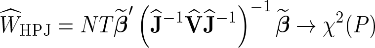
{\hat{W}}_{HPJ} = N T {\tilde{β}}^{'} {({\hat{J}}^{- 1} \hat{V} {\hat{J}}^{- 1})}^{- 1} \tilde{β} \to χ^{2} (P)

where $\hat{J} = {(N T)}^{- 1} \sum_{i = 1}^{N} X_{i}^{'} M_{Z_{i}} X_{i}$ .

When the errors are assumed to be homoskedastic along both time and crosssectional dimensions, then

\hat{V} = {\hat{σ}}^{2} \hat{J}

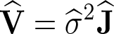
with the variance estimator given by

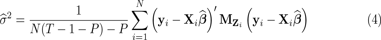
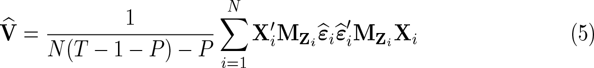
{\hat{σ}}^{2} = \frac{1}{N (T - 1 - P) - P} \sum_{i = 1}^{N} {(y_{i} - X_{i} \hat{β})}^{'} M_{Z_{i}} (y_{i} - X_{i} \hat{β})

On the other hand, if the errors are cross-sectionally heteroskedastic,

\hat{V} = \frac{1}{N (T - 1 - P) - P} \sum_{i = 1}^{N} X_{i}^{'} M_{Z_{i}} {\hat{ε}}_{i} {\hat{ε}}_{i}^{'} M_{Z_{i}} X_{i}

The model in (1) can allow for weak cross-section dependence as in Sarafidis and Wansbeek (2012) and Dumitrescu and Hurlin (2012). Under weak cross-sectional dependence, the HPJ estimator $\hat{β}$ remains consistent, but $\hat{V}$ in the above equations is not. In this case, an estimator for $\hat{V}$ is obtained by using the pairs bootstrap as in Gonçalves and Kaffo (2015). Unreported Monte Carlo simulations show that this approach works well in finite samples.

3 The xtgrangert command

3.1 Syntax

xtgrangert depvar [indepvars ] [if] [in] [, lags( # ) maxlags( # ) het nodfc bootstrap[( #reps , seed( seed ))] sum]

Data must be xtset before using xtgrangert. The panel must be balanced.

3.2 Options

lags( # ) specifies the number of lags of dependent and independent variables to be added to the regression. The default is lags(1). The lags of the dependent variable are partialed out.

maxlags( # ) specifies the upper bound of lags. The BIC is used to select the number of lags that provides the best model fit. lags() and maxlags() cannot be used at the same time.

het allows for cross-sectional heteroskedasticity.

nodfc does not apply the degrees-of-freedom correction in (4) and (5). This option is mostly useful under cross-sectional heteroskedasticity.

bootstrap[( #reps , seed( seed ))] specifies a bootstrap variance estimator in the HPJ Wald statistic that allows for cross-sectional dependence and uses a custom seed and #reps replications. By default, 100 replications are used based on the current seed. This is useful in the presence of weak cross-sectional dependence.

sum presents results on the sum of the estimated feedback coefficients. This option can be useful when P > 1.

3.3 Stored results

xtgrangert stores the following in e():

3.4 Postestimation command

predict can be used after xtgrangert. The syntax for predict is

predict newvar [if] [in] [, residuals xb]

residuals calculates the residuals.

xb calculates the linear prediction on the partialed-out variables.

4 Example

4.1 Estimation of the determinants of banks’ capital adequacy ratios

To illustrate the xtgrangert command, we perform Granger noncausality tests and examine the type of temporal relation between profitability, cost efficiency, and asset quality in the U.S. banking industry. We draw a random sample of 450 U.S. bankholding companies, each one observed over 56 time periods, namely, 2006:Q1–2019:Q4. The data are publicly available, and they have been downloaded from the Federal Deposit Insurance Corporation website.⁵

We focus on the following model,

\begin{array}{l} RO A_{i, t} = ϕ_{0, i} + \sum_{p = 1}^{P} ϕ_{p, i} RO A_{i, t - p} + \sum_{p = 1}^{P} β_{1, p, i} inefficienc y_{i, t - p} \\ + \sum_{p = 1}^{P} β_{2, p, i} qualit y_{i, t - p} + ε_{i, t} \end{array}

for i = 1,…, N(= 450) and t = P + 1,…, T (= 56).

ROA _i,t stands for the “return on assets” and is used as a measure of profitability; in particular, it is defined as annualized net income expressed as a percentage of average total assets. inefficiency _i,t ₋ _p presents a measure of cost inefficiency, which has been constructed from a stochastic cost frontier model using a translog function form.⁶ Finally, quality _i,t ₋ _p represents the quality of banks’ assets and is computed as the total amount of loan-loss provisions expressed as a percentage of assets. Thus, a higher level of loan-loss provisions indicates lower quality.

We start by testing whether the pair of inefficiency and quality Granger-causes ROA. Then, we consider univariate tests by modeling ROA as a function of inefficiency and quality separately. Throughout, we allow for a maximum of four lags of the dependent variable and the covariates. The following results are obtained:

As we can see, the null hypothesis that cost inefficiency and asset quality do not Granger-cause profitability is rejected at the 5% level of significance. The optimal number of lags equals 1 according to the BIC.⁷ The option het requests computing cross-sectional heteroskedasticity-robust standard errors.

In addition to the Wald test statistic, the command also reports regression results with respect to the HPJ bias-corrected pooled estimator. The regression output above indicates that the test outcome may be driven by inefficiency. To shed some light on this issue, we test for Granger noncausality for each variable separately using univariate tests. We obtain the following output:

The output on the top (bottom) corresponds to the Granger noncausality univariate test of the relationship between profitability and cost inefficiency (asset quality). The null hypothesis that inefficiency does not Granger-cause ROA is rejected at the 5% level of significance. This implies that past values of inefficiency contain information that helps to predict ROA over and above the information contained in past values of ROA. On the other hand, one fails to reject the null hypothesis that quality does not Granger-cause ROA.

To illustrate further options of the xtgrangert command, we split the sample into two groups according to their asset size, where the partitioning is determined based on the kmeans clustering algorithm available in Stata. Subsequently, we test for Granger noncausality for the smallest banks in the sample, using data from 2011:Q1 onward, which corresponds to quarter 1 of the first year following the enactment of the Dodd– Frank Wall Street Reform and Consumer Protection Act of 2010.⁸ We obtain the following results:

As before, the null hypothesis that inefficiency and quality do not Grangercause ROA is rejected at the 5% level of significance. Note that the optimal number of lags equals 2. The option sum requests reporting the sum of the lags of the regression coefficients for each variable.

5 Conclusions

xtgrangert implements the Granger noncausality test of Juodis, Karavias, and Sarafidis (2021). The command reports the Wald test statistic and its p-value, the null and the alternative hypotheses, and regression results with respect to the HPJ bias-corrected pooled estimator. The command offers options for both manual and automatic laglength selection, using a BIC. Moreover, the command allows for cross-section dependence and cross-section heteroskedasticity in the errors.

The Granger causality testing approach developed by Juodis, Karavias, and Sarafidis (2021) is computationally fast and widely applicable. In the presence of cross-section dependence, some caution must be exercised with interpreting the results. This is because we do not provide a formal proof that the bootstrap methodology used in this article is asymptotically valid in this case. The same issue applies to other notable contributions in the literature; see, for example, Dumitrescu and Hurlin (2012). While the Monte Carlo simulations are encouraging, a formal investigation on the properties of estimators and the bootstrap is an interesting direction for future research.

A special case of strong cross-section dependence is the additive time effect of the two-way fixed effects model, which is frequently used in the literature. Typically, this time effect is removed by transforming the data to deviations from their cross-sectional means for each time period. This approach is valid if the panel is assumed to be homogeneous across i. After the transformation, the Juodis, Karavias, and Sarafidis (2021) test can be applied without using the bootstrap. If, however, the panel is heterogeneous, then the demeaning no longer removes the additive time effect.

7 Programs andx supplemental materials

Supplemental Material, sj-zip-1-stj-10.1177_1536867X231162034 - Improved tests for Granger noncausality in panel data

Supplemental Material, sj-zip-1-stj-10.1177_1536867X231162034 for Improved tests for Granger noncausality in panel data by Jiaqi Xiao, Yiannis Karavias, Artūras Juodis, Vasilis Sarafidis and Jan Ditzen in The Stata Journal

Footnotes

6 Acknowledgments

Financial support from the Netherlands Organization for Scientific Research (NWO) under research grant number 451-17-002 is gratefully acknowledged by Artūras Juodis. Jan Ditzen acknowledges financial support from the Italian Ministry MIUR under the PRIN project Hi-Di NET—Econometric Analysis of High Dimensional Models with Network Structures in Macroeconomics and Finance (grant 2017TA7TYC).

7 Programs andx supplemental materials

To install a snapshot of the corresponding software files as they existed at the time of publication of this article, type

The xtgrangert command also is available on the Statistical Software Components Archive and can be installed directly in Stata with the command

. ssc install xtgrangert

Notes

References

Abrigo

M. R. M.

Love

2016. Estimation of panel vector autoregression in Stata. Stata Journal 16: 778–804. https://doi.org/10.1177/1536867X1601600314.

Bun

M. J. G.

Sarafidis

2015. Dynamic panel data models. In The Oxford Handbook of Panel Data, ed. Baltagi

B. H.

, 76–110. Oxford: Oxford University Press. https://doi.org/10.1093/oxfordhb/9780199940042.013.0003.

Dhaene

Jochmans

2015. Split-panel jackknife estimation of fixed-effect models. Review of Economic Studies 82: 991–1030. https://doi.org/10.1093/restud/rdv007.

Dufour

J.-M.

Renault

1998. Short run and long run causality in time series: Theory. Econometrica 66: 1099–1125. https://doi.org/10.2307/2999631.

Dumitrescu

E.-I.

Hurlin

2012. Testing for Granger non-causality in heterogeneous panels. Economic Modelling 29: 1450–1460. https://doi.org/10.1016/j.econmod.2012.02.014.

Emirmahmutoglu

Kose

2011. Testing for Granger causality in heterogeneous mixed panels. Economic Modelling 28: 870–876. https://doi.org/10.1016/j.econmod.2010.10.018.

Fernández-Val

Lee

2013. Panel data models with nonadditive unobserved heterogeneity: Estimation and inference. Quantitative Economics 4: 453–481. https://doi.org/10.3982/QE75.

Gonçalves

Kaffo

2015. Bootstrap inference for linear dynamic panel data models with individual fixed effects. Journal of Econometrics 186: 407–426. https://doi.org/10.1016/j.jeconom.2015.02.017.

Granger

C. W. J.

1969. Investigating causal relations by econometric models and crossspectral methods. Econometrica 37: 424–438. https://doi.org/10.2307/1912791.

10.

Holtz-Eakin

Newey

Rosen

H. S.

1988. Estimating vector autoregressions with panel data. Econometrica 56: 1371–1395. https://doi.org/10.2307/1913103.

11.

Juodis

Karavias

Sarafidis

2021. A homogeneous approach to testing for Granger non-causality in heterogeneous panels. Empirical Economics 60: 93–112. https://doi.org/10.1007/s00181-020-01970-9.

12.

Juodis

Sarafidis

2022. An incidental parameters free inference approach for panels with common shocks. Journal of Econometrics 229: 19–54. https://doi.org/10.1016/j.jeconom.2021.03.011.

13.

Karavias

Tzavalis

2016. Local power of fixed-T panel unit root tests with serially correlated errors and incidental trends. Journal of Time Series Analysis 37: 222–239. https://doi.org/10.1111/jtsa.12144.

14.

Karavias

Tzavalis

2017. Local power of panel unit root tests allowing for structural breaks. Econometric Reviews 36: 1123–1156. https://doi.org/10.1080/07474938.2015.1059722.

15.

Lopez

Weber

2017. Testing for Granger causality in panel data. Stata Journal 17: 972–984. https://doi.org/10.1177/1536867X1801700412.

16.

Sarafidis

Wansbeek

2012. Cross-sectional dependence in panel data analysis. Econometric Reviews 31: 483–531. https://doi.org/10.1080/07474938.2011.611458.

17.

Wursten

2018. Testing for serial correlation in fixed-effects panel models. Stata Journal 18: 76–100. https://doi.org/10.1177/1536867X1801800106.

Supplementary Material

Please find the following supplemental material available below.

For Open Access articles published under a Creative Commons License, all supplemental material carries the same license as the article it is associated with.

For non-Open Access articles published, all supplemental material carries a non-exclusive license, and permission requests for re-use of supplemental material or any part of supplemental material shall be sent directly to the copyright owner as specified in the copyright notice associated with the article.

0.58 MB

0.00 MB