Sage Journals: Discover world-class research

Abstract

Recently, a new statistical methodology to assess the bias and precision of a new measurement method, which circumvents the deficiencies of the Bland and Altman (1986, Lancet 327: 307–310) limits of agreement method, was developed by Taffé (2018, Statistical Methods in Medical Research 27: 1650–1660). Later, the methodology was extended to assess the agreement. In addition, to allow for inferences, simultaneous confidence bands around the bias, precision, and agreement lines were developed (Taffé, 2020, Statistical Methods in Medical Research 29: 778–796). The goal of this article is to introduce the extended biasplot command, which implements these latest developments, and to illustrate its use by applying it to simulated data included with the command. Note that the Taffé method assumes that there are several measurements by one of the two measurement methods and possibly as few as one measurement by the other for each individual. The repeated measurements need not come from the reference standard but from any of the two measurement methods. This is a great advantage because it may sometimes be more feasible to gather repeated measurements either with the reference standard or the new measurement method.

Keywords

gr0068_1 biasplot agreement bias precision limits of agreement differential bias proportional bias method comparison

1 Introduction

In clinical research, Bland and Altman’s limits of agreement (LoA) method is frequently used to assess the agreement or interchangeability between two measurement methods, when the characteristic of interest is continuous (Altman and Bland 1983; Bland and Altman 1986). Often, this is motivated by a new, perhaps less expensive or easier, method of measurement against an established reference standard. To evaluate the comparability of the methods, the investigator collects measurements, perhaps one or several, from each method for a set of subjects. Bland and Altman’s LoA are then computed by adding and subtracting 1.96 times the estimated standard deviation (SD) from the mean differences. A scatterplot of the differences versus the means of the two variables with the LoA superimposed is used to visually appraise the degree of agreement and quantify the magnitude. Further, a regression of the differences as a function of the means is added to the plot to indicate whether there is a bias and the direction of that bias (Bland and Altman 1999).

Bland and Altman’s plot may be misleading, however, in situations where the variances of the measurement error for each method differ from one another. When this is the case, the regression line may show an upward or downward trend when there is no bias or a zero slope when there is a bias (Carstensen 2010; Taffé 2018).

Recently, a new statistical methodology to assess the bias and precision of a new measurement method, which circumvents the deficiencies of the Bland and Altman’s LoA method, was developed (Taffé 2018). Later, that methodology was extended to include the assessment of the agreement, and the inference was developed to build simultaneous confidence bands (CBs) around the bias, precision, and agreement lines (Taffé 2020).

In this article, we will present the implementation of the extended methods proposed by Taffé (2020). A series of new graphs will be introduced to help the investigator assess bias, precision, and agreement between the different measurement methods. The methodology requires repeated measurements on each individual for at least one of the two measurement methods (otherwise, one cannot identify the differential and proportional biases). It was originally developed based on repeated measurements from the reference standard, but it has been extended to the setting where repeated measurements come from the new measurement method (however, this option has not been implemented in the current command and has to be done manually). This is a great advantage because it may sometimes be more feasible to gather repeated measurements with the new measurement method.

The extended biasplot command now includes an option to allow the user to save the results of the estimation procedure and build plots including several competitive measurement methods. Thanks to the simultaneous CBs, inference can be carried out for the whole curve and is not limited to only a specific value of the latent trait (as with pointwise CBs).

2 The measurement error model

2.1 Formulation and estimation of the model

Following Taffé (2018), we define the relationship between the true latent trait, x_ij , and the measured outcomes, y ₁ _ij (by method 1) and y ₂ _ij (by method 2), on individual i at measurement j, by

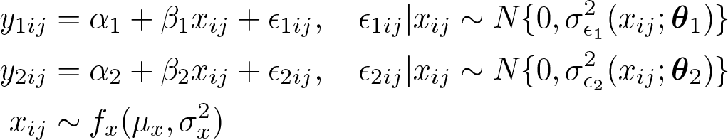
\begin{array}{l} y_{1 i j} = α_{1} + β_{1} x_{i j} + ϵ_{1 i j}, ϵ_{1 i j} ∣ x_{i j} ~ N {0, σ_{ϵ_{1}}^{2} (x_{i j}; θ_{1})} \\ y_{2 i j} = α_{2} + β_{2} x_{i j} + ϵ_{2 i j}, ϵ_{2 i j} ∣ x_{i j} ~ N {0, σ_{ϵ_{2}}^{2} (x_{i j}; θ_{2})} \\ x_{i j} ~ f_{x} (μ_{x}, σ_{x}^{2}) \end{array}

where ϵ ₁ _ij and ϵ ₂ _ij are the measurement errors by methods 1 and 2 and f_x is the density of the true unknown trait. The parameters α ₁ and α ₂ measure the differential bias, whereas β ₁ and β ₂ the proportional bias. This formulation makes it clear that neither method 1 nor method 2 needs to be unbiased. The goal is to compare the two measurement methods and assess the bias of one of the two versus the other (which will be called the “reference method” whether genuinely unbiased or not).

For the sake of clarity, we now consider method 2 to be the reference standard and method 1 the new method to be evaluated. We also assume that the individual latent trait is constant within individual i; that is, x_ij ≡ x_i , although this assumption could be relaxed (Taffé 2018). Therefore, the model reduces to

\begin{array}{l} y_{1 i j} = α_{1} + β_{1} x_{i} + ϵ_{1 i j}, ϵ_{1 i j} ∣ x_{i} ~ N {0, σ_{ϵ_{1}}^{2} (x_{i}; θ_{1})} \\ y_{2 i j} = x_{i} + ϵ_{2 i j}, ϵ_{2 i j} ∣ x_{i} ~ N {0, σ_{ϵ_{2}}^{2} (x_{i}; θ_{2})} \\ x_{i} ~ f_{x} (μ_{x}, σ_{x}^{2}) \end{array}

and α ₁ measures the differential and β ₁ the proportional bias relative to measurement method 2. We assume that there are replicate measurements j = 1,…, n_i on each individual i, i = 1,…, N, by at least one of the two measurement methods and that the variances $σ_{ϵ_{1}}^{2}$ (x_i ; θ ₁) and $σ_{ϵ_{2}}^{2}$ (x_i ; θ ₂), which depend on vectors of unknown parameters, θ ₁ and θ ₂, are heteroskedastic and depend on the level of the true latent trait, x_i , by the relationships

\begin{array}{l} σ_{ϵ_{1}} (x_{i}; θ_{1}) = (θ_{1}^{(0)} + θ_{1}^{(1)} x_{i}) \sqrt{π / 2} \\ σ_{ϵ_{2}} (x_{i}; θ_{2}) = (θ_{2}^{(0)} + θ_{2}^{(1)} x_{i}) \sqrt{π / 2} \end{array}

Actually, the form of the heterogeneity need not be a straight line, and a fractional polynomial may be used instead if the investigator believes that the straight-line model is too restrictive. The presence of the square root term $\sqrt{π / 2}$ is related to the halfnormal distribution of the absolute value of the residuals.

Taffé (2018) has developed a two-step procedure to estimate the parameters of (2) and (2), which does not rely on the density of the true unknown trait, f_x . Simulations have shown that this two-step approach works well to estimate the differential and proportional biases, even with as few as three to five repeated measurements by one of the two methods and only one by the other.

When the repeated measurements are available for method 1 instead of method 2 (the reference), the two-step procedure operates the same way as in Taffé (2018), except that the role of y ₂ _ij is taken by y ₁ _ij and computation of the differential and proportional biases is modified accordingly. That is, in this case, the user proceeds by first fitting a regression model for y ₁ _ij by marginal maximum likelihood. Then, the mean of the conditional distribution of x_i given the vector y ₁ _i is computed, and the regression model $y_{2 i j} = α + β \hat{E} (x_{i} ∣ y_{1 i}) + ϵ_{2 i j}$ estimated by ordinary least squares. Therefore, the differential bias is given by −α/β, and proportional bias by 1/β. Finally, the best linear unbiased prediction (BLUP) of x_i is simply computed as ${\hat{x}}_{i} = \hat{α} + \hat{β} \hat{E} (x_{i} ∣ y_{1 i})$ . Based on the estimated parameters and their estimated variance–covariance matrix, inference regarding the differential and proportional bias can be carried out by using the delta method.

When repeated measurements are available for both measurement methods, the user may start in the two-step procedure by fitting a regression model for either y ₂ _ij or y ₁ _ij . The estimates of the differential and proportional biases will be similar (but not the same). Our experience, along with limited simulations, suggests that it is advantageous to use the method having on average more repeated measurements as the reference (confidence intervals [CIs] are slightly narrower).

The (total) bias $E (y_{1 i j} - y_{2 i j} | x_{i})$ is consistently estimated by

{bias}_{i} = {\hat{α}}_{1}^{*} + {\hat{x}}_{i} ({\hat{β}}_{1}^{*} - 1)

where ${\hat{α}}_{1}^{*}$ and ${\hat{β}}_{1}^{*}$ are estimates from the linear regression model of the new measurement method y ₁ _ij on the BLUP ${\hat{x}}_{i}$ ; that is, $y_{1 i j} = α_{1}^{*} + β_{1}^{*} {\hat{x}}_{i} + ϵ_{1 i j}^{*}$ .

2.2 Inference

Taffé (2020) developed a new methodology to allow the computation of simultaneous CBs around the bias (3) and each of the two SD (2) lines. The simultaneous CB approach guarantees a proper coverage rate for the simultaneous inference, whatever the number of points from the support considered. It therefore allows proper inference for the whole curve, whereas a pointwise CI guarantees that on average, only 95% of the computed intervals for each individual point from the support will cover the true value. The latter is appropriate only when the focus is on a single point (that is, value) from the latent trait but not for the whole curve.

Note that in the presence of a proportional bias, the new measurement method needs to be recalibrated, using $y_{1 i j}^{*} = (y_{1 i j} - {\hat{α}}_{1}) / {\hat{β}}_{1}$ , before proceeding to the comparison of the precisions of the two methods (Taffé 2018). Indeed, in the presence of a proportional bias, there is a scale issue without recalibration, because the latter acts multiplicatively on the true trait. This means that y ₁ and y ₂ are not on the same scale. This is akin to the situation where one instrument measures a distance in meters and the other in feet; like is not compared with like without recalibration (Taffé 2021).

2.3 The mean squared error

As mentioned above, in the presence of a proportional bias, method 1 is not on the same scale as method 2; therefore, the variances of the measurement errors of the two instruments may not be compared without recalibration. However, if the user does not want to recalibrate method 1, then the mean squared errors (MSEs) may be compared instead of the SDs. As method 2 is the reference, its MSE equals its variance, ${MSE}_{2} = {({\hat{θ}}_{2}^{(0)} + {\hat{θ}}_{2}^{(1)} {\hat{x}}_{i})}^{2} π / 2$ , whereas for method 1, the user has to compute

{MSE}_{1} = {({\hat{θ}}_{1}^{(0)} + {\hat{θ}}_{1}^{(1)} {\hat{x}}_{i})}^{2} π / 2 + {{\hat{α}}_{1}^{*} + {\hat{x}}_{i} ({\hat{β}}_{1}^{*} - 1)}^{2}

The user can compute 95% simultaneous CBs for MSE₁ and MSE₂ exactly in the same way as for the bias and the SD (Taffé 2020). Alternatively, the user may similarly compute the square root MSE to produce a figure in the same units as the reference standard.

2.4 The agreement

To assess the agreement between the two measurement methods, following a similar path as Bland and Altman, Taffé (2020) defines the α-level upper and lower limits of agreement ${LoA}_{α}^{up}$ and ${LoA}_{α}^{lo}$ as

{LoA}_{α} = E (y_{1 i j} - y_{2 i j} ∣ x_{i}) \pm Z_{1 - α / 2} \sqrt{V (y_{1 i j} - y_{2 i j} ∣ x_{i})}

where the conditional distribution of the differences, d_ij = y ₁ _ij − y ₂ _ij |x_i , is assumed to be normally distributed. The main difference between the Bland and Altman approach and the Taffé approach is that the Taffé methodology conditions on x_i to resolve the issue of endogeneity and allow the variances to be heteroskedastic and depend on the level x_i of the true latent trait.

The LoA are estimated by

est. {LoA}_{α} = {bias}_{i} \pm Z_{1 - α / 2} \sqrt{{\hat{σ}}_{d}^{2}}

where the estimate of the variance $σ_{d}^{2}$ of the differences is given by

{\hat{σ}}_{d}^{2} \equiv \hat{V} (y_{1 i j} - y_{2 i j} ∣ x_{i}) = {\hat{σ}}_{ϵ_{1}}^{2} ({\hat{x}}_{i}; {\hat{θ}}_{1}) + {\hat{σ}}_{ϵ_{2}}^{2} ({\hat{x}}_{i}; {\hat{θ}}_{2})

Simultaneous 95% CBs for ${LoA}_{α}^{up}$ and ${LoA}_{α}^{lo}$ are computed in the same way as above for the bias and two SDs.

2.5 The percentage of agreement

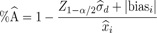
To assess the level of agreement between the two measurement methods, Taffé (2020) has developed a new index, the “percentage of agreement”, defined by (in terms of a proportion)

% A = 1 - \frac{Z_{1 - α / 2} SD (y_{1 i j} - y_{2 i j} ∣ x_{i}) + | E (y_{1 i j} - y_{2 i j} ∣ x_{i}) |}{x_{i}}

where Z ₁ _−α _/ ₂ is the 1 − α/2 percentile point of the standard normal distribution. Note that for (4), the percentage of agreement is defined by the percentage of disagreement, captured by the fraction portion of the above equation. In the numerator, the 1 − α/2 percentile point Z ₁ _−α _/ ₂SD(y ₁ _ij −y ₂ _ij |x_i ) of the conditional distribution of the differences y ₁ _ij − y ₂ _ij (which is assumed to be normally distributed) is penalized by the absolute value of the bias and then divided by the value of the latent trait. Finally, one minus the fraction represents the percentage of agreement. Notice that the percentage of agreement may turn out to be negative whenever the numerator is larger than the denominator, in which case the agreement is extremely poor.

The original intention of Bland and Altman (1983, 1986), when they developed the LoA plot, was that it was up to the investigator to appraise the level of agreement between the two measurement methods, which is deliberately subjective. However, as an aid to interpreting results and because the agreement may not be constant over the whole support, we have developed the “percentage of agreement”, which is based on a formula.

The percentage of agreement is computed as

% \hat{A} = 1 - \frac{Z_{1 - α / 2} {\hat{σ}}_{d} + | {bias}_{i} |}{{\hat{x}}_{i}}

When method 1 has been recalibrated (to remove the bias), the user uses the “corrected percentage of agreement” instead:

% A^{*} = 1 - \frac{Z_{1 - α / 2} SD (y_{1 i j}^{*} - y_{2 i j} ∣ x_{i})}{x_{i}}

which is estimated by

% {\hat{A}}^{*} = 1 - \frac{Z_{1 - α / 2} {\hat{σ}}_{d^{*}}}{{\hat{x}}_{i}}

Again, simultaneous 95% CBs for %A, respectively %A^∗, can be computed as above for the bias and two SDs.

3 The extended biasplot command

The extended biasplot command extends the previous biasplot command by integrating the computation of the newly proposed parameters, that is, MSE, ${LoA}_{α}^{up}$ and ${LoA}_{α}^{lo}$ , percentage of agreement %A, and corrected percentage of agreement %A ^∗ . In addition, simultaneous CBs are computed around each parameter and a series of new graphs can be drawn (the total bias, agreement without recalibration, agreement after recalibration, percentage agreement without recalibration, percentage agreement after recalibration, MSE, and squared root MSE plots) to help the investigator to assess bias, precision, and agreement between the two measurement methods.

3.1 Syntax

The syntax for biasplot is the same as in the previous version of the command (Taffé et al. 2017), except that there are additional options.

biasplot [if] [in], idvar( varname ) ynew( varname ) yref( varname ) [loa bias totbias precision comp agreement0 agreement1 pctagreement0 pctagreement1 mse sqrtmse results pdfs nbsimul( # ) ]

3.2 Options

idvar( varname ) defines the variable identifying the individual. idvar() is required.

ynew( varname ) defines the new measurement method. ynew() is required.

yref( varname ) defines the reference standard method. yref() is required.

loa graphs the extended LoA plot. Note that you have to choose at least one of the options loa , bias , totbias , precision , etc. for the command to run and save the corresponding graphs to the current directory.

bias graphs the bias plot.

totbias graphs the total bias plot.

precision graphs the precision plot.

comp graphs the comparison plot.

agreement0 graphs the agreement plot without recalibration.

agreement1 graphs the comparison plot after recalibration.

pctagreement0 graphs the percentage agreement plot without recalibration.

pctagreement1 graphs the percentage agreement plot after recalibration.

mse graphs the MSE plot.

sqrtmse graphs the square root MSE plot.

results generates a file called biasplot _results.dta containing the original data plus the estimates computed by the command (all the variables are prefixed by my_ varname ) .

pdfs saves the graphs in .pdf format (instead of Stata’s .gph format).

nbsimul( # ) allows the user to change the default value (that is, nbsimul(1000) ) of the number of simulations carried out to compute the CBs. For example, to set the number of simulations to 2,000, use the option nbsimul(2000) .

3.3 Stored results

biasplot stores the following in r() :

4 Numerical examples

To illustrate the use of the extended biasplot command, we will consider three simulated datasets.

4.1 Simulation model 1

\begin{array}{l} y_{1 i} = 4 + 0.8 x_{i} + ϵ_{1 i}, ϵ_{1 i} ∣ x_{i} ~ N {0, {(0.2 x_{i})}^{2}} \\ y_{2 i j} = x_{i} + ϵ_{2 i j},_{2 i j} ∣ x_{i} ~ N {0, {(1.75 + 0.08 x_{i})}^{2}} \\ x_{i} ~ Uniform [25 - 45] \end{array}

where i = 1,…, 100, and the number of repeated measurements of individual i from the reference standard was n ₂ _i ∼ Uniform[10−20] and n ₁ _i ∼ Uniform[1−3] for the new measurement method.

There are between 10 and 20 repeated measurements by the reference standard and between 1 and 3 by the new measurement method for each individual. The new method (method 1) has a differential bias of 4 and a proportional bias of 0.8. In addition, the variance of the measurement errors from method 1 is larger than that of the reference method 2. Notice that as the individuals do not have the same number of observations, the precision of the prediction (BLUP of x) of the latent trait will vary across individuals, and a smoothing of the CBs has been implemented using fractional polynomials of degree 2.

The data have been saved in the file named biasplot _example_data_set1.dta .

We load the example dataset 1:

. use biasplot_example_data_set1

We call the biasplot command with the options loa and bias :¹

Figure 1.

(a) Standard Bland and Altman LoA plot and (b) bias plot

Based on Taffé’s (2018) methodology, a differential bias of 3.5 (true value 4), 95% CI = [−1.87; 8.80], and a proportional bias of 0.82 (true value 0.8), 95% CI = [0.66; 0.97], are identified, whereas with the standard Bland and Altman methodology, a differential bias of −9.0 (true value 4), 95% CI = [−17.7; −0.4], and a proportional bias of 1.16 (true value 0.8), 95% CI = [0.96; 1.36], are found.

The bias plot may seem complicated to read at first sight because it has two y axes, but it is, in fact, a standard scatterplot. The left y axis represents the values (y ₁ and y ₂) of the measurements made by the two instruments, whereas the x axis represents the true value of the latent trait after measurement errors have been removed (more precisely, it is the best possible estimation of the latent trait, that is, BLUP). Therefore, the bias plot is simply a scatterplot of the measurements, y ₁ and y ₂, with the x axis representing the true latent trait. In Bland and Altman’s LoA plot, the true value of the trait is estimated by the mean of the two measurements, that is, (y ₁ + y ₂)/2, whereas in the bias plot, it is estimated using all the measurements of the individuals.

By inspecting the bias plot (shown here in grayscale), we see that the regression line of the new method y ₁ (green in the actual plot) lies below the one of the reference y ₂ (black) for all the values of the true latent trait. Clearly, the method y ₁ has a negative bias over the whole support from 25 to 45. The bias of the method y ₁ is equal to the vertical distance between the green line and the black one. Because it is difficult to read this distance directly on the plot, the bias plot has a second y axis on the right. This right y axis works like a magnifying glass and shows the distance between the two lines. For example, when the true trait is 45, the distance between the green and black lines is about −5, as can be read on the right y axis using the red bias line. Likewise, when the true trait is 25, the distance between the green and black regression lines is about −1 (here the magnifying glass is really useful because it is difficult to read the distance between the two lines directly on the scatterplot).

This example clearly illustrates a setting where Bland and Altman’s methodology provides biased and misleading results, whereas the “bias plot” methodology shows that the bias of the new method is larger the higher the latent trait.

We will present below the newly proposed graphs to help the investigator to assess bias, precision, and agreement between the two measurement methods. These may be obtained by running the biasplot command four separate times to get each of the total bias, precision, agreement0 , and agreement1 plots,

or, more compactly, by using a single command:

In both situations, the four graphs are saved in the current directory, but in the latter situation, only the last figure will be open:

Figure 2.

(a) Total bias plot with simultaneous CBs; (b) precision plot with simultaneous CBs; (c) agreement plot without recalibration; and (d) agreement plot after recalibration

The total bias plot focuses on the (total) bias, which results from the two components of bias: the differential and proportional biases. It works as a magnifying glass of the bias line from the bias plot. The simultaneous CBs around the total bias line allow the user to formally assess whether bias is statistically significant and on which portion of the support.

The precision plot with its simultaneous CBs around the two SD lines allows the user to formally compare the precision of the two instruments under consideration (there is a statistically significant difference between 30 and 45), after recalibration of the new measurement method to resolve the scaling issue.

The agreement plot is similar to the classical Bland and Altman LoA plot, except that the x axis is the predicted true latent trait (that is, BLUP of x) instead of the mean of the two measurements. It allows the user, by inspecting the lower and upper limits, while accounting for the CBs, to visually and quantitatively (by reading the percentage of agreement on the right y axis) appraise the degree of agreement between the two measurement methods. Without recalibration, the LoA are centered on the bias line, whereas they are centered on the zero value after recalibration. After method 1 has been recalibrated, and the differential and proportional biases removed, the line of bias is confounded with the x axis, and the agreement plot shows that agreement is better for higher values of the latent trait.

The reading of the percentage of agreement is not always easy on the agreement plot, and no CB appears around the percentage of agreement index. To inspect thoroughly the percentage of agreement, the user may compute the “percentage of agreement” plots, using the commands

Figure 3.

(a) Percentage of agreement plot without recalibration and (b) percentage of agreement plot after recalibration

The percentage of agreement plot allows for a formal assessment of the level of agreement. When there are three or more measurement methods to be compared, the percentage of agreement plot may turn out to be useful for formally comparing the levels of the agreement by superimposing the curves along with their simultaneous CBs on the same plot (illustrated below).

Because of the scale issue, in the presence of a proportional bias, the new measurement method was recalibrated before computing the SD of the measurement errors. However, if the user is reluctant to perform a recalibration and prefers to conserve the measurements by method 1 as is (despite a bias), then he or she may compare the precision of the two measurement methods using the MSE (to account for the bias) or the square root MSE (to produce a figure in the same units as the reference standard) instead of the SD:

Figure 4.

(a) The MSE plot illustrates that the MSE of method 1 tends to be larger than that of method 2, although not statistically significant as the CBs’ overlap over the whole support; and (b) the MSE plot produces a figure in the same units as the reference standard.

Comparison of the MSE plot with the precision plot (compare with figure 2) reveals that, after we removed the bias from method 1, the precision of method 2 turned out to be clearly superior to that of method 1 almost over the whole support, whereas this was not as apparent on the MSE plot or its square root counterpart.

4.2 Illustration of the results option

Another feature we have added to this extended version of the biasplot command is the results option, which allows the user to retrieve the estimates. For example, to retrieve the estimate of the total bias, we type

which will generate a file called biasplot _results.dta containing the original data plus the estimates computed by the command (all the variables are prefixed by my_ varname ) . To illustrate, we have generated two additional datasets.

4.3 Simulation model 2

This dataset is based on the same simulation model (5), except we have increased the number of repeated measurements by the new method y ₁, that is, n ₁ _i Uniform[10−20], and widened the support x_i ∼ Uniform[20−100] to allow easier reading of the plots.

The data have been saved in the file named biasplot _example_data_set2.dta .

4.4 Simulation model 3

\begin{array}{l} y_{1 i} = 1 + 0.9 x_{i} + ϵ_{1 i}, ϵ_{1 i} ∣ x_{i} ~ N {0, {(1 + 0.04 x_{i})}^{2}} \\ y_{2 i j} = x_{i} + ϵ_{2 i j}, ϵ_{2 i j} ∣ x_{i} ~ N {0, {(1.75 + 0.08 x_{i})}^{2}} \\ x_{i} ~ Uniform [20 - 100] \end{array}

with n ₂ _i ∼ Uniform[10−20] and n ₁ _i ∼ Uniform[10−20]. The simulated data have been saved in the file named biasplot _example_data_set3.dta .

Notice that, in this dataset, we did not use the same values of the reference method as in the first simulation dataset. Rather, new values were simulated using the same model because we wanted to mimic the setting where the reference method had been used twice in two separate experiments but on the same population, with two different new measurement methods to be compared.

Consider, first, the comparison of the two total bias plots:

Figure 5.

(a) The total bias plot from simulation model (5) and (b) total bias plot from simulation model (6)

These two total bias plots may be combined using the following code:

Figure 6.

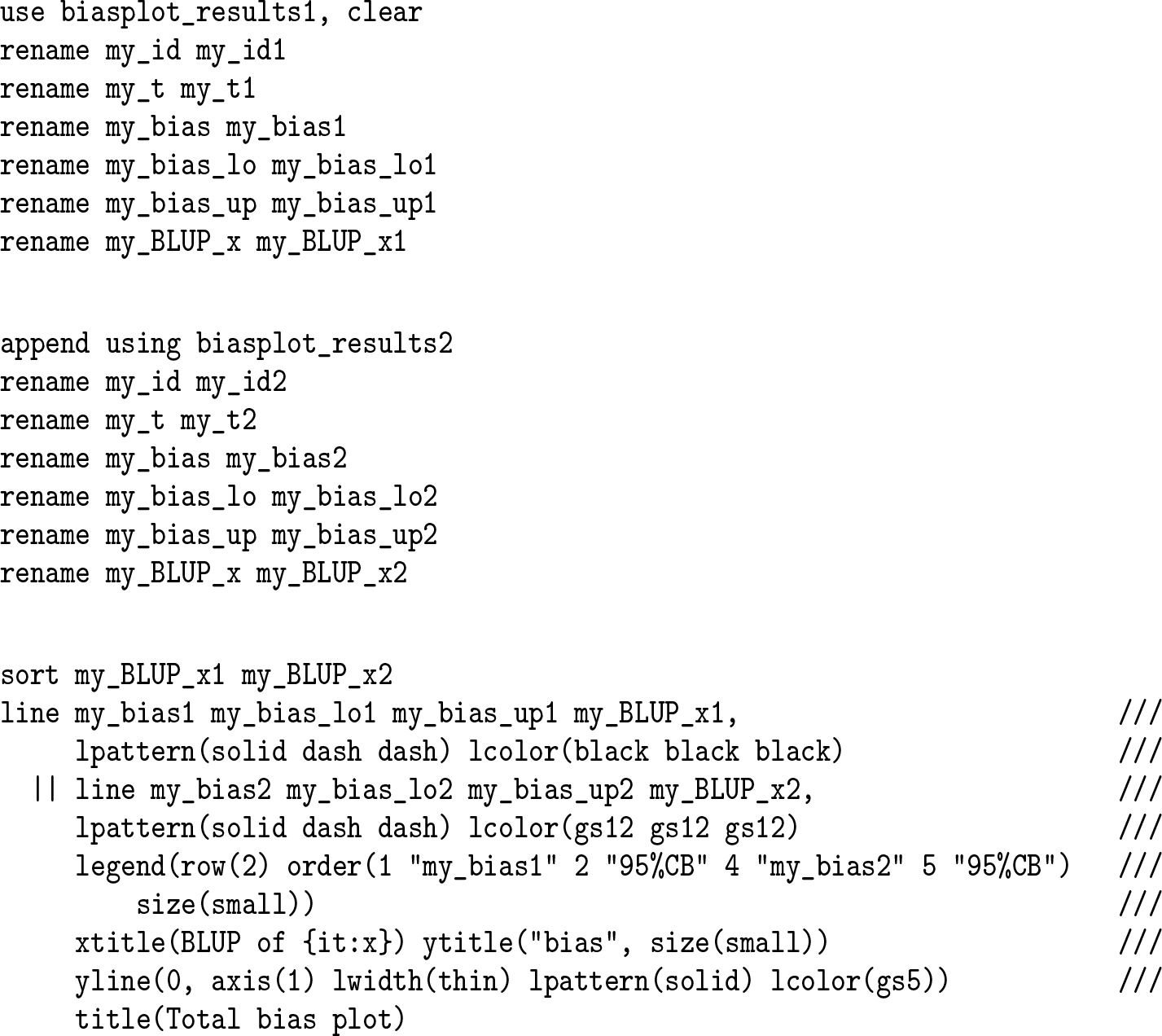
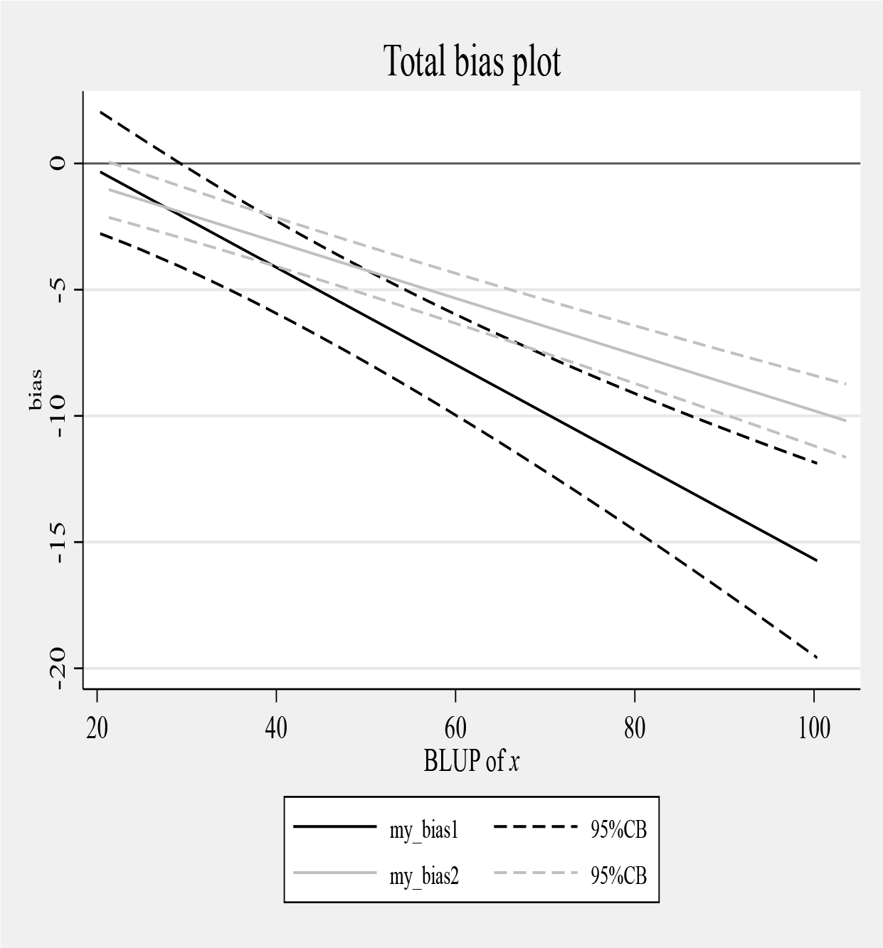
Total bias plot combining bias estimates from simulation models (5) and (6)

From 70, measurement method 2 has a lower bias than method 1.

Now we will consider the comparison of the two precision plots:

Figure 7.

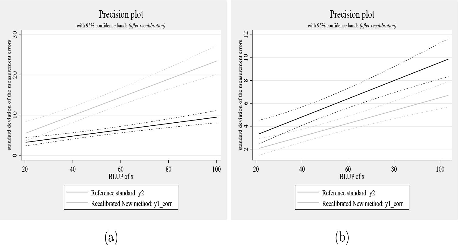
(a) The precision plot from simulation model (5) and (b) precision plot from simulation model (6)

These two precision plots may be combined using the following code:

Figure 8.

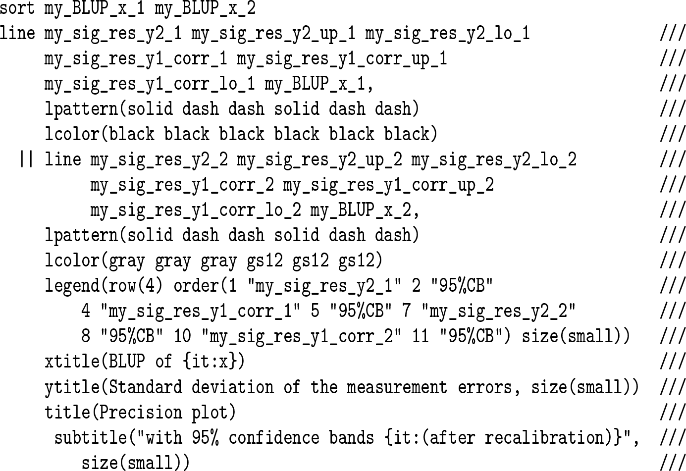
Total bias plot combining bias estimates from simulation models (5) and (6)

Clearly, after recalibration, measurement method 1 (my_sig_res_y1_corr_1 ) from the simulation model (5) is less precise than reference method 2 (my_sig_res_y2_1 ), and measurement method 2 (my_sig_res_y1_corr_2 ) from the simulation model (6) is more precise than reference method 2 (my_sig_res_y2_2 ). Additionally, the user may observe that the two reference SD lines, along with their 95% CBs, that is, reference method 2 (my_sig_res_y2_1 ) from the simulation model (5) and reference method 2 (my_sig_res_y2_2 ) from the simulation model (6), are similar (but not exactly the same), which was expected given that the two samples have been simulated by the same model.

5 Discussion

Based on simulated data, we have illustrated the use of the extended biasplot command to assess bias, precision, and agreement between two measurement methods. The current version of the command implements simultaneous CBs around each parameter computed to allow formal inferences. This is particularly relevant from a clinical perspective. For example, thanks to the simultaneous CB around the total bias line, one can assess the amount of bias of the new measurement method for any value or over any interval of values of the predicted latent trait (that is, BLUP of x), which is not the case with pointwise CBs. This is useful because it may turn out that the bias is statistically significant only for large values of the latent trait, in which case without recalibration, the instrument may be safely used for low values but not for large ones.

Also, by superimposing the bias lines and simultaneous CBs obtained from several new measurement methods on the same plot, the user may assess which method performs best in terms of bias according to the level of the latent trait (note that this is not implemented in the current biasplot command, but users may generate the figure by using the saved estimates in biasplot _results.dta ). Similarly, by superimposing the estimated SD curves and simultaneous CBs obtained from several new measurement methods on the same plot, the user may determine which method (after recalibration) is more precise in which range of the latent trait. If the investigator is reluctant to recalibrate the new measurement method, he or she may use the MSE plot or, better, the square root MSE plot instead.

The agreement plot is similar to the standard Bland and Altman LoA plot (Bland and Altman 1986), except that its x axis is the BLUP of the true latent trait and not the average of the two measurements (as in the Bland and Altman LoA plot). It is as simple to read and interpret as the traditional LoA plot but has the additional advantage of including on the right y axis a quantitative summary index of the degree of agreement. Having a quantitative index in addition to the plot may greatly help the interpretation of the results. As for the bias and precision plots, the user may draw on the same plot the percentage agreement and CB computed for different measurement methods. This provides a convenient way to compare the level of agreement between different competitive measurement methods.

In our experience, to get a reasonable estimate of the precision (that is, the SD of the measurement errors), at least 8 to 10 repeated measurements by one of the two measurement methods are needed. Note that the repeated measurements need not be from the reference standard. This is a great asset of our methodology because sometimes it may turn out to be easier to perform many measurements by the new measurement method. Requiring repeated measurements by one of the two methods might discourage the applied researcher to use our methodology. However, this is necessary for statistical identification. Indeed, when the variance of the measurement errors of each measurement method is not constant or their ratio is unknown, which is usually the case in the biomedical field (the variance of measurement errors often increases as the latent trait increases), having only one measurement by each of the two measurement methods does not allow the user to identify the bias (Dunn 2004).

When the focus is mainly on estimation of the differential and proportional biases, as few as three to five repeated measurements from the reference standard and only one measurement by the new method, or vice versa, is required to get good estimates (Taffé 2020).

Note that our modeling technique rests on the assumption that the individual latent trait is constant within individuals; that is, x_ij ≡ x_i . This means that the repeated measurements should ideally be taken in sequence within a time interval where this assumption is sensible. For example, in our application to systolic blood pressure data, the measurements were taken in sequence with 30 seconds between each measurement, and the assumption of an average constant latent blood pressure was sensible (Taffé, Halfon, and Halfon 2020). It is theoretically possible to extend the methodology to other settings where the latent trait has a time trend (Taffé 2018). However, in that case, the simple and convenient decomposition of the bias into (constant) differential and proportional components is probably not sensible, and more sophisticated models should be developed.

6 Conclusions

In conclusion, the extension of the biasplot command provides investigators with a whole array of new figures to assess bias, precision, and agreement between two measurement methods. Thanks to the simultaneous CBs, it allows the user to formally compare several competing measurement methods. The methodology rests on the assumption that the individual latent trait is constant within individuals, which is an assumption that must be carefully considered. In particular, the repeated measurements should, when possible, be taken at reasonably not too long time intervals for the assumption to be sensible. To get reasonable estimates of the precision, one must use at least 8 to 10 repeated measurements by one of the two measurement methods, whereas when the focus is mainly on the differential and proportional biases, as few as 3 to 5 repeated measurements from the reference standard and only one by the new method, or vice versa, will do.

8 Programs and supplemental materials

Supplemental Material, sj-zip-1-stj-10.1177_1536867X231161978 - Extended biasplot command to assess bias, precision, and agreement in method comparison studies

Supplemental Material, sj-zip-1-stj-10.1177_1536867X231161978 for Extended biasplot command to assess bias, precision, and agreement in method comparison studies by Patrick Taffé, Mingkai Peng, Vicki Stagg and Tyler Williamson in The Stata Journal

Footnotes

7 Declaration of conflicting interests

The authors declare no potential conflicts of interest with respect to the research, authorship, or publication of this article.

8 Programs and supplemental materials

To install a snapshot of the corresponding software files as they existed at the time of publication of this article, type

Notes

References

Altman

D. G.

Bland

J. M.

1983. Measurement in medicine: The analysis of method comparison studies. Journal of the Royal Statistical Society, Series D 32: 307–317. https://doi.org/10.2307/2987937.

Bland

J. M.

Altman

D. G.

1986. Statistical methods for assessing agreement between two methods of clinical measurement. Lancet 327: 307–310. https://doi.org/10.1016/S0140-6736(86)90837-8.

Bland

J. M.

Altman

D. G.

. 1999. Measuring agreement in method comparison studies. Statistical Methods in Medical Research 8: 135–160. https://doi.org/10.1177/096228029900800204.

Carstensen

2010. Comparing methods of measurement: Extending the LoA by regression. Statistics in Medicine 29: 401–410. https://doi.org/10.1002/sim.3769.

Dunn

2004. Statistical Evaluation of Measurement Errors: Design and Analysis of Reliability Studies. 2nd ed. London: Arnold.

Steichen

T. J.

Cox

N. J.

2002. A note on the concordance correlation coefficient. Stata Journal 2: 183–189. https://doi.org/10.1177/1536867X0200200206.

Taffé

2018. Effective plots to assess bias and precision in method comparison studies. Statistical Methods in Medical Research 27: 1650–1660. https://doi.org/10.1177/0962280216666667.

Taffé

. 2020. Assessing bias, precision, and agreement in method comparison studies. Statistical Methods in Medical Research 29: 778–796. https://doi.org/10.1177/0962280219844535.

Taffé

2021. When can the Bland & Altman limits of agreement method be used and when it should not be used. Journal of Clinical Epidemiology 137: 176–181. https://doi.org/10.1016/j.jclinepi.2021.04.004.

10.

Taffé

Halfon

2020. A new statistical methodology overcame the defects of the Bland–Altman method. Journal of Clinical Epidemiology 124: 1–7. https://doi.org/10.1016/j.jclinepi.2020.03.018.

11.

Taffé

Peng

Stagg

Williamson

2017. biasplot: A package to effective plots to assess bias and precision in method comparison studies. Stata Journal 17: 208–221. https://doi.org/10.1177/1536867X1701700111.

Supplementary Material

Please find the following supplemental material available below.

For Open Access articles published under a Creative Commons License, all supplemental material carries the same license as the article it is associated with.

For non-Open Access articles published, all supplemental material carries a non-exclusive license, and permission requests for re-use of supplemental material or any part of supplemental material shall be sent directly to the copyright owner as specified in the copyright notice associated with the article.

0.12 MB

0.00 MB

Extended biasplot command to assess bias,precision,and agreement in method comparison studies

Abstract

Keywords

1 Introduction

2 The measurement error model

2.1 Formulation and estimation of the model

2.2 Inference

2.3 The mean squared error

2.4 The agreement

2.5 The percentage of agreement

3 The extended biasplot command

3.1 Syntax

3.2 Options

3.3 Stored results

4 Numerical examples

4.1 Simulation model 1

4.2 Illustration of the results option

4.3 Simulation model 2

4.4 Simulation model 3

5 Discussion

6 Conclusions

8 Programs and supplemental materials

Supplemental Material, sj-zip-1-stj-10.1177_1536867X231161978 - Extended biasplot command to assess bias, precision, and agreement in method comparison studies

Footnotes

7 Declaration of conflicting interests

8 Programs and supplemental materials

Notes

References

Supplementary Material