robustpf: A command for robust estimation of production functions

Abstract

We introduce a new command, robustpf, to estimate parameters of Cobb–Douglas production functions. The command is robust against two potential problems. First, it is robust against optimization errors in firms’ input choice, unobserved idiosyncratic cost shocks, and measurement errors in proxy variables. In particular, the command relaxes the conventional assumption of scalar unobservables. Second, it is also robust against the functional dependence problem of static input choice, which is known today as a cause of identification failure. The main method is proposed by Hu, Huang, and Sasaki (2020, Journal of Econometrics 215: 375–398).

1 Introduction

Empirical analysis of production functions is relevant to a wide range of economic fields, including industrial organization, international trade, macroeconomics, and the economics of education. Although production is one of the most primitive components of economic structures, identification and estimation of production functions from observational data are known to be delicate and difficult.

Simultaneity in the choice of input factors is one of the major sources of the difficulty (Marschak and Andrews 1944). To date, a number of solutions have been proposed to solve this problem. One of the most widely used econometric methods today is the control function approach proposed by Olley and Pakes (1996) and Levinsohn and Petrin (2003), which is implemented by the levpet (Petrin et al. 2004) and prodest (Rovigatti and Mollisi 2018) commands.

The control function approach often uses the investment or an intermediate input factor as a proxy of productivity. In many instances, however, these proxy variables are subject to unobserved errors, which may stem from firms’ optimization errors, unobserved idiosyncratic cost shocks, or measurement errors. While this additional randomness imposes more difficulty, Hu, Huang, and Sasaki (2020) show that the production function parameters may be still identified under this extended setting. This article introduces the robustpf command to implement the robust estimation method proposed by Hu, Huang, and Sasaki (2020).

This article is organized as follows. Section 2 discusses a model of production. Section 3 reviews Hu, Huang, and Sasaki’s (2020) estimation method. Section 4 describes the syntax and options for robustpf. Section 5 illustrates the command, using panel data for Chilean firms. Section 6 concludes.

2 The model of production

We consider the general structural framework like that in Olley and Pakes (1996) and consider the Cobb–Douglas production function of the form

$y_t={\beta }_k{k}_t+l_t{\beta }_l+m_t{\beta }_m+{\omega }_t+{\eta }_t$

1

where y_t denotes the logarithm of the output, k_t denotes the logarithm of the capital input, l _t denotes the row vector of the logarithms of the labor inputs, m _t denotes the row vector of the logarithms of intermediate inputs, ω_t denotes the logarithm of the latent productivity that subsumes the constant term and follows the first-order Markov process E(ω_t |ω_{t − 1}) = ρ(ω_{t − 1}), and η_t denotes the idiosyncratic shock with E(η_t |k_t, l _t, m _t, ω_t ) = 0. We are interested in estimating the parameter vector ${\left({\beta }_k,{\beta }_l^{\prime },{\beta }_m^{\prime }\right)}^{\prime }$ in this model. The vector l _t may include multiple types of labor such as skilled labor $l_t^s$ and unskilled labor $l_t^u$ , and the vector m _t may also include multiple kinds of intermediate input such as materials $m_t^1$ , electricity $m_t^2$ , and fuel $m_t^3$ .

Each firm makes a decision about the capital input k_t in period t−1 before observing the innovation ω_t −E(ω_t |ω_{t − 1}) in productivity. Specifically, k_t follows the law of motion

$\begin{array}{c}{k}_t=\kappa \left(k_{t-1},i_{t-1},{\nu }_{t-1}\right)\\ i_t={\iota }_t\left(k_t,{\omega }_t,{\zeta }_t\right)\end{array}$

where i_t denotes the logarithm of investment and (ν_{t − 1} , ζ_t )′ captures unobserved factors. Then, each firm makes a decision about the static input (l _t, m _t )′ simultaneously in period t, after observing (k_t, ω_t )′ by solving the static optimization problem

$\underset{\left(l_t,m_t\right)}{\max }\exp \left({\beta }_k{k}_t+l_t{\beta }_l+m_t{\beta }_m+{\omega }_t+{\eta }_t\right)-\left\{\exp \left(l_t\right)p_l+\exp \left(m_t\right)p_m\right\}$

where p _l and p _m denote the vectors of the prices of exp(l _t ) and exp(m _t ), respectively. This static part of the firm’s problem yields the reduced-form input choice rules of the linear form

$x_t={\mathit{\text{α}}}_x{ }_0+{\mathit{\text{α}}}_{xk}{k}_t+{\mathit{\text{α}}}_{x\omega }{\omega }_t+p_t{\mathit{\text{α}}}_{xp}$

for each input coordinate x of l and m. This kind of choice rule leads to the functional dependence problem, where the static input x_t by construction has no source of variations freely from the variations of the state variables (k_t, ω_t )′ and thus fails the identification in general (Ackerberg, Caves, and Frazer 2015, sec. 3).

To solve this problem of identification failure, we generalize the above input choice rule to

$x_t={\mathit{\text{α}}}_x{ }_0+{\mathit{\text{α}}}_{xk}{k}_t+{\mathit{\text{α}}}_{x\omega }{\omega }_t+{ϵ}_{xt}$

2

where ε_xt is a scalar random variable that is unobserved by a researcher. This error term can be interpreted as a result of the firm’s optimization error, unobserved idiosyncratic cost shocks, and measurement error by a researcher—see Hu, Huang, and Sasaki (2020, sec. 2.4.1). While this extended input choice rule (2) certainly solves the aforementioned functional dependence problem, the additional unobserved randomness in ε_xt may potentially cause the identification problem to be even more difficult. Yet using the spectral decomposition approach, Hu, Huang, and Sasaki (2020) show that the production function parameters ${\left({\beta }_k,{\beta }_l^{\prime },{\beta }_m^{\prime }\right)}^{\prime }$ may be identified under suitable conditions—in fact, they show more general nonparametric identification. While we omit the details of the identification argument here, we refer readers to section 2.2 in Hu, Huang, and Sasaki (2020). In light of this identification result, we can now consistently estimate the production function parameters ${\left({\beta }_k,{\beta }_l^{\prime },{\beta }_m^{\prime }\right)}^{\prime }$ . The following section reviews the estimation method from section 3 of Hu, Huang, and Sasaki (2020).

3 Review of the estimation method

For convenience of writing, we write the Cobb–Douglas production function in logarithms (1) more succinctly as

${\tilde{y}}_t(\beta )={\omega }_t+{\eta }_t$

where $\beta ={\left({\beta }_k,{\beta }_l^{\prime },{\beta }_m^{\prime }\right)}^{\prime }$ and $y{e}_t(\beta )\equiv y_t-({\beta }_k{k}_t+l_t{\beta }_l+m_t{\beta }_m)$ . Likewise, we write the reduced-form demand functions for static input in logarithms (2) as

${\tilde{x}}_{t+1}\left({\mathit{\text{α}}}_x\right)={\mathit{\text{α}}}_{x\omega }{\omega }_{t+1}+{ϵ}_{xt+1}$

where ${\mathit{\text{α}}}_x= ({\mathit{\text{α}}}_x{ }_0, {\mathit{\text{α}}}_{xk})$ and ${\tilde{x}}_{t+1}\left({\mathit{\text{α}}}_x\right)$ $\equiv x_t{ }_{+1}-({\mathit{\text{α}}}_x{ }_0+{\mathit{\text{α}}}_{xk}{k}_t{ }_{+1})$ . Let the Markov process of the productivity ω_t be given by the polynomial

$\rho \left({\omega }_{t-1}\right)={\displaystyle \sum _{p=1}^P{\rho }_p}{\omega }_{t-1}^p$

of degree P for some natural number P to be specified by a researcher. Finally, we write the random vector ez _t ≡ (i_t, k_t, l _t, m _t )′ and the reduced-form parameter ϕ_q = α_{x ω}ρ_q for each q = 1,…, P .

Under these notations, Hu, Huang, and Sasaki (2020, sec. 3) derive the moment restrictions of the form

$E\left[{\tilde{z}}_t\left\{{\tilde{x}}_{t+1}\left({\mathit{\text{α}}}_x\right)-{\displaystyle {\sum }_{p=1}^P{\phi }_p}{\tilde{y}}_t{(\beta )}^p\right\}\right]=0,\text{\hspace{1em}\hspace{0.17em}\hspace{0.17em}for\hspace{0.17em}}P\le 2$

for any proxy x. For the case of P > 2, we need to introduce additional notations to succinctly write moment restrictions. Let

$M(t,P)=\left(\begin{array}{cccc}1& & & \\ \left(\begin{array}{l}2\hfill \\ 1\hfill \end{array}\right)E\left({\eta }_t\right)& 1& & \\ ⋮& ⋮& \ddots & \\ \left(\begin{array}{l}P\hfill \\ 1\hfill \end{array}\right)E\left({\eta }_t^{P-1}\right)& \left(\begin{array}{l}P\hfill \\ 2\hfill \end{array}\right)E\left({\eta }_t^{P-2}\right)& \cdots & 1\end{array}\right)$

and ${\tilde{\phi }}_p:={\displaystyle {\sum }_{q=1}^P{\phi }_q}{\left\{M{(t,P)}^{-1}\right\}}_{(q,p)}$ for p = 1,…, P . We then have the moment restrictions of the form

$E\left[{\tilde{z}}_t\left\{{\tilde{x}}_{t+1}\left({\mathit{\text{α}}}_x\right)-{\displaystyle {\sum }_{p=1}^P{\tilde{\phi }}_p{\tilde{y}}_t{(\beta )}^p}\right\}\right]=0$

3

for any proxy x. Similarly, we can obtain additional moment restrictions of the form

$E\left[{\tilde{z}}_t\left\{{\tilde{y}}_{t+1}\left({\mathit{\text{α}}}_x\right)-{\displaystyle {\sum }_{p=1}^P{\mathit{\text{α}}}_{x\omega }^{-1}{\tilde{\phi }}_p{\tilde{y}}_t{(\beta )}^p}\right\}\right]=0$

4

Now, write the moment restrictions (3) and (4) as E{g _t ( θ )}, where

$g_t(\mathit{\text{θ}})=\left(\begin{array}{l}{\tilde{z}}_t\left\{{\tilde{y}}_{t+1}\left({\mathit{\text{α}}}_x\right)-{\displaystyle {\sum }_{p=1}^P{\mathit{\text{α}}}_{x\omega }^{-1}{\tilde{\phi }}_p{\tilde{y}}_t{(\beta )}^p}\right\}\hfill \\ {\tilde{z}}_t\left\{{\tilde{x}}_{t+1}\left({\mathit{\text{α}}}_x\right)-{\displaystyle {\sum }_{p=1}^P{\tilde{\phi }}_p{\tilde{y}}_t{(\beta )}^p}\right\}\hfill \end{array}\right)$

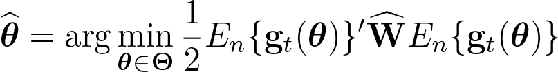
and $\mathit{\text{θ}}={\left({\mathit{\text{α}}}_x^{\prime },{\mathit{\text{α}}}_{x\omega },{\beta }^{\prime },{\tilde{\phi }}_1,\dots ,{\tilde{\phi }}_P\right)}^{\prime }$ . For a suitable weighting matrix $\widehat{W}$ , the generalized method of moments (GMM) estimator $\widehat{\mathit{\text{θ}}}$ for θ is defined by

$\widehat{\mathit{\text{θ}}}=\arg \underset{\mathit{\text{θ}}\in \Theta }{\min }\frac{1}{2}{E}_n{\left\{g_t(\mathit{\text{θ}})\right\}}^{\prime }\widehat{W}{E}_n\left\{g_t(\mathit{\text{θ}})\right\}$

where E_n denotes the cross-sectional sample mean operator. The robustpf command uses the identity matrix for the weighting matrix $\widehat{W}$ in the first step of its GMM estimation and the estimated efficient weighting matrix $\widehat{W}$ in the second step of its GMM estimation. As with the usual GMM routines, the robustpf command approximates the variance of $\sqrt{n}(\widehat{\mathit{\text{θ}}}-\mathit{\text{θ}})$ by the following:

$\widehat{V}={\left({\widehat{G}}^{\prime }\widehat{W}\widehat{G}\right)}^{-1}{\widehat{G}}^{\prime }\widehat{W}\widehat{\Sigma }\widehat{W}\widehat{G}{\left({\widehat{G}}^{\prime }\widehat{W}\widehat{G}\right)}^{-1}$

$\widehat{G}=E_n\left\{D_{\mathit{\text{θ}}}{g}_t(\widehat{\mathit{\text{θ}}})\right\}$ is an estimator of G = E{D _θ g _t ( θ ₀)} and $\widehat{\Sigma }=E_n\left\{g_t(\widehat{\mathit{\text{θ}}})g_t(\widehat{\mathit{\text{θ}}}{)}^{\prime }\right\}$ is an estimator of Σ = E{g _t ( θ ₀)g _t ( θ ₀)′}. D _θ denotes the gradient operator.

Finally, we note that Hu, Huang, and Sasaki (2020) present extensive Monte Carlo simulation studies in their section 3.3, where they compare the estimation method proposed above against existing alternatives (Olley and Pakes 1996; Levinsohn and Petrin 2003; Wooldridge 2009) under many scenarios. In the following section, we introduce the robustpf command, which produces $\widehat{\mathit{\text{θ}}}$ and $\widehat{V}$ defined above.

4 The robustpf command

The robustpf command is an e-class command.

4.1 Syntax

The syntax of the robustpf command is as follows.

robustpf depvar [if] [in], capital( varname ) free( varlist ) proxy( varname ) [m( varlist ) onestep dfp bfgs init_capital( real ) init_free( real ) init_m( real )]

Here depvar denotes the logarithm of the output y_t ; the capital() option sets the logarithm of the capital input k_t ; the free() option sets the logarithms of one or more types of labor input l _t ; and the proxy() option sets a proxy variable. Exactly one depvar, exactly one capital() variable, at least one free() variable, and exactly one proxy() variable should be included to run the command. For analysis of gross-output production functions, the logarithms of one or more types of intermediate input m _t can be set with the m() option.

4.2 Options

capital( varname ) takes a state input variable, such as capital. capital() is required. free( varlist ) takes free input variables, such as labor.

free() is required. proxy( varname ) takes the proxy variable used for estimation of the production function. proxy() is required.

m( varlist ) takes intermediate input variables for estimation of the gross-output production function. By default, the command estimates the net-output production function.

onestep sets an indicator for implementing just one step of the GMM estimation. By default, two-step efficient GMM estimation is set.

dfp sets an indicator for implementing the Davidon–Fletcher–Powell optimization algorithm. By default, the Newton–Raphson method is set.

bfgs sets an indicator for implementing the Broyden–Fletcher–Goldfarb–Shanno optimization algorithm. By default, the Newton–Raphson method is set.

init_capital( real ) sets the initial value of the capital coefficient for an optimization routine of the GMM estimation. The default is init_capital(0.1).

init_free( real ) sets the initial values of the labor coefficients for an optimization routine of the GMM estimation. The default is init_free(0.1).

init_m( real ) sets the initial values of the intermediate input coefficients for an optimization routine of the GMM estimation. The default is init_m(0.3).

The moment function for GMM estimation is nonlinear. Therefore, we recommend trying multiple initial values to improve the chance of attaining the globally optimal solution. The value of the objective is stored in e(objective) after running the command to compare local solutions.

4.3 Stored results

The robustpf command stores the following results in e():

5 Illustration of the command

This section illustrates the robustpf command. We use panel data for Chilean firms, consisting of food manufacturing plants (ISIC code: 311) from 1981 to 1983. The data come from the census for plants collected by Chile’s Instituto Nacional de Estadistica. This panel dataset has been used by many important articles on productivity analysis, including the seminal article by Levinsohn and Petrin (2003). See Lui (1991) for detailed descriptions of data construction.

To proceed with analysis, we first load the dataset by the following command line.

. use example_chile

The panel data consist of 994 firms (cross-sectional units) for 7 years (time periods). This is an unbalanced panel with a total of 5,566 observations. The firm identifier is stored in the variable named id. The year identifier is stored in the variable named year. Prior to running the robustpf command, we first set these panel dimensions by using the xtset command as follows.

. xtset id year

(output omitted)

For analysis of net output production functions, we include the capital and labor factors but do not include an intermediate input. A proxy variable is required to control for the unobserved productivity. Common choices of a proxy variable include the investment (as in Olley and Pakes [1996]) and an intermediate input (as in Levinsohn and Petrin [2003]). Suppose that we include the capital k, skilled labor ls, and unskilled labor lu as factors of production and use the material m() as a proxy for productivity. Recall that the method implemented by the robustpf command is robust against optimization errors, idiosyncratic cost shocks, and measurement errors in the intermediate input choice m(). In this setting, the net output production function

$y_t={\beta }_k{k}_t+{\beta }_{l^s}{l}_t^s+{\beta }_{l^u}{l}_t^u+{\beta }_m{m}_t+{\omega }_t+{\eta }_t$

can be estimated by running

Output of the robustpf command shows a panel for Chilean firms, consisting of food manufacturing plants (ISIC code: 311) from 1981 to 1983. Displayed are coefficient estimates for the capital, skilled labor, and unskilled labor in the net-output production function, along with their standard errors, z ratios, p-values, and confidence intervals.

Also displayed above the table of the main results is an estimate of the returns to scale, computed as the sum of the three coefficient values, along with its standard error. Observe that this net output production function entails a significantly positive elasticity for each of the two types of labor input and also exhibits constant returns to scale in the sense that the returns are not significantly different from one.

We next compare these estimation results of robustpf with those of the most popular alternatives from the existing literature. First, we run the prodest (Rovigatti and Mollisi 2018) command to implement an estimation based on the method of Levinsohn and Petrin (2003)—see also Petrin, Poi, and Levinsohn (2004). Specifically, following Petrin, Poi, and Levinsohn (2004, sec. 4), but still using the same dataset as above, we run the following two command lines.

. tsset id year

(output omitted)

. prodest y, free(ls lu) state(k) proxy(m) va met(lp) id(id) t(year)

(output omitted)

Second, we also obtain estimates based on the method of Wooldridge (2009). To this end, we use the prodest command as follows.

. prodest y, free(ls lu) state(k) proxy(m) va met(wrdg) id(id) t(year)

(output omitted)

Finally, we again run the prodest command, but this time to obtain estimates based on the method of Levinsohn and Petrin (2003) along with the correction by Ackerberg, Caves, and Frazer (2015) as follows.

. prodest y, free(ls lu) state(k) proxy(m) va met(lp) acf id(id) t(year)

(output omitted)

The following table compares their estimation results with those of robustpf based on Hu, Huang, and Sasaki (2020).

In the first row of table 1, LP yields small point estimates for both of the two labor coefficients, ls and lu. Adding up all the three coefficient estimates together yields the estimated returns to scale of 0.638. This number indicates strongly diminishing returns to scale. The estimates presented in the second row of table 1, based on W, show a pattern similar to the LP estimates presented in the first row. This similarity is a natural outcome because LP and W use the same set of identifying moment restrictions, and their estimation strategies differ only in that W implements a simultaneous estimation (to obtain accurate standard errors) of the two-step estimator, while LP implements a procedural estimation.

Table 1.

Estimation results by the methods of Levinsohn and Petrin (LP, 2003), Wooldridge (W, 2009), Ackerberg, Caves, and Frazer (ACF, 2015) correction of LP, and Hu, Huang, and Sasaki (HHS, 2020). The results are based on a panel for Chilean firms, consisting of food manufacturing plants (ISIC code: 311) from 1981 to 1983.

Method	Command	Coefficients			Returns to scale	Test of constant returns to scale
		k	ls	lu
LP	prodest	0.279 (0.016)	0.132 (0.009)	0.227 (0.008)	0.638 (0.032)	Reject; diminishing returns
W	prodest	0.184 (0.045)	0.140 (0.023)	0.228 (0.020)	0.552 (0.047)	Reject; diminishing returns
ACF	prodest	0.310 (0.018)	0.385 (0.002)	0.496 (0.007)	1.191 (0.010)	Reject; increasing returns
HHS	robustpf	0.082 (0.062)	0.402 (0.043)	0.486 (0.042)	0.969 (0.142)	Fail to reject; constant returns

In the third row of table 1, the method of LP with the ACF correction yields substantially larger point estimates for both of the two labor coefficients than those of LP or W presented in the first two rows. These large differences come from a modified set of moment restrictions proposed by ACF to circumvent the identification failure of the LP method due to the functional dependence problem—see ACF (2015, sec. 3). Adding up all the three coefficient estimates of ACF together yields the estimated returns to scale of 1.191, which is now larger than 1 and is significantly different from 1. In other words, the estimates based on the method of ACF imply strongly increasing returns to scale in contrast to the diminishing returns implied by LP and W.

Finally, we present the estimates based on our proposed robustpf command in the bottom row of table 1 shown in the output of robustpf on page 92. The point estimates of the two labor coefficients are similar to those of ACF. On the other hand, the point estimate of the capital coefficient is smaller than that of ACF. Consequently, adding up all three coefficient estimates of HHS together yields the estimated returns to scale of 0.969, which is not significantly different from 1. Therefore, the estimates by the robustpf command based on the method of HHS are consistent with constant returns to scale unlike estimation results of the other three methods. This difference may be explained by the fact that ACF requires the conventional assumption of scalar unobservables, while HHS does not require this restriction. Alternatively, this difference may also stem from the restriction on the input demand function that the method of HHS uses in addition to the structural restrictions on the output equation.

6 Conclusion

In this article, we introduced a new command, robustpf, that estimates parameters of Cobb–Douglas production functions with robustness against optimization errors in firms’ input choice, unobserved idiosyncratic cost shocks, and measurement errors in proxy variables. The command is based on the method of Hu, Huang, and Sasaki (2020). As a by-product of introducing and allowing for errors in the static input choices, the command is also robust against the functional dependence problem, which Ackerberg, Caves, and Frazer (2015) pointed out as a cause of identification failure in general. Thus, the robustpf command provides users with robustness against two potential problems with production function estimation.

In closing this article, we discuss a limitation of the command. The method of estimation is based on the nonlinear GMM criterion presented in section 3, and thus numerical methods are not guaranteed to find the global optimum. The default algorithm of the command is the Newton–Raphson method, and section 3.2 presents a couple of alternative options. We recommend that a user run several estimates with different initial values of optimization by using the options to set initial values presented in section 3.2. The value of the GMM objective achieved at the local optimum can be retrieved from e(objective), and a user can compare the optimal criterion values associated with different estimates. This practical inconvenience can be overcome if a global optimization routine is developed for implementation of robustpf. We leave it for future research.

7 Programs and supplemental materials

Supplemental Material, sj-zip-1-stj-10.1177_1536867X231161977 - robustpf: A command for robust estimation of production functions

Supplemental Material, sj-zip-1-stj-10.1177_1536867X231161977 for robustpf: A command for robust estimation of production functions by Yingyao Hu, Guofang Huang and Yuya Sasaki in The Stata Journal

References

1.
AckerbergD. A.CavesK.FrazerG.2015. Identification properties of recent production function estimators. Econometrica83: 2411–2451. https://doi.org/10.3982/ECTA13408.
2.
HuY.HuangG.SasakiY.2020. Estimating production functions with robustness against errors in the proxy variables. Journal of Econometrics215: 375–398. https://doi.org/10.1016/j.jeconom.2019.05.024.
3.
LevinsohnJ.PetrinA.2003. Estimating production functions using inputs to control for unobservables. Review of Economic Studies70: 317–341. https://doi.org/10.1111/1467-937X.00246.
4.
LuiL.1991. Entry-exit and productivity changes: An empirical analysis of efficiency frontiers. PhD thesis, University of Michigan. https://hdl.handle.net/2027.42/128821.
5.
MarschakJ.AndrewsW. H.Jr.1944. Random simultaneous equations and the theory of production. Econometrica12: 143–205. https://doi.org/10.2307/1905432.
6.
OlleyG. S.PakesA.1996. The dynamics of productivity in the telecommunications equipment industry. Econometrica64: 1263–1297. https://doi.org/10.2307/2171831.
7.
PetrinA.PoiB. P.LevinsohnJ.2004. Production function estimation in Stata using inputs to control for unobservables. Stata Journal4: 113–123. https://doi.org/10.1177/1536867X0400400202.
8.
RovigattiG.MollisiV.2018. Theory and practice of total-factor productivity estimation: The control function approach using Stata. Stata Journal18: 618–662. https://doi.org/10.1177/1536867X1801800307.
9.
WooldridgeJ. M.2009. On estimating firm-level production functions using proxy variables to control for unobservables. Economics Letters104: 112–114. https://doi.org/10.1016/j.econlet.2009.04.026.
Supplementary Material
Please find the following supplemental material available below.
For Open Access articles published under a Creative Commons License, all supplemental material carries the same license as the article it is associated with.
For non-Open Access articles published, all supplemental material carries a non-exclusive license, and permission requests for re-use of supplemental material or any part of supplemental material shall be sent directly to the copyright owner as specified in the copyright notice associated with the article.