Sage Journals: Discover world-class research

Abstract

In some applications, only a coarsened version of a categorical outcome variable can be observed. Parametric inference based on the maximum likelihood approach is feasible in principle, but it cannot be covered computationally by standard software tools. In this article, we present two commands facilitating maximum likelihood estimation in this situation for a wide range of parametric models for categorical outcomes—in the cases both of a nominal and an ordinal scale. In particular, the case of probabilistic information about the possible values of the outcome variable is also covered. Two examples motivating this scenario are presented and analyzed.

Keywords

st0668 pccfit pccprob coarsened data multinomial distribution multinomial regression ordinal outcome variables ordered regression human osteoarchaeology palaeodemography diagnostic accuracy studies imperfect reference standard

1 Introduction

1.1 Background

In some applications, only a coarsened version C of a categorical outcome variable Y can be observed; that is, C is a subset of all categories indicating the “possible” values of Y but including in any case the true value of Y. The theory of fitting a parametric model $p_{θ}^{Y}$ from (partially) coarsened observations is well developed (Heitjan and Rubin 1991; Gill, van der Laan, and Robins 1997), making use of the classical maximum-likelihood (ML) principle and focusing on the coarsened at random (CAR) situation. In this article, we consider mainly the case that additional information is available about how Y is actually distributed across the categories of C, based on some additional information E. To be precise, we assume that P (Y |C, E) is known under the assumption of a certain distribution for Y.

We start with presenting two examples motivating this setup. Next, we establish the likelihood for C, and we present the commands pccfit and pccprob to compute ML estimates and model-based estimates of class probabilities, respectively. We then tackle several questions originating in the two examples to illustrate the use of the commands. We finish with a discussion about alternatives and issues related to the use of pccfit.

1.2 Motivating example 1: Coarsened age categories in human osteoarchaeology

Analyzing former populations represented by human skeletal remains excavated from archaeological sites is a core task of human osteoarchaeology (White, Black, and Folkens 2011). Determining age and sex of each skeletal individual is usually the first basic step, allowing researchers to describe the demographic structure (age and sex distribution) of the skeletal population. Skeletal age determination is based on traits that become fully expressed only around a certain age in infancy or adolescence or that change or degenerate during adulthood. Because of the variability in physical development, determining the exact, that is, chronological, age is not feasible, and the use of classification systems with classes like infant, juvenile, adult, mature, and senile is common. But even with such categories, often an individual’s age cannot be determined with sufficient precision to be attributed to a single category or class, and only two or more possible categories can be determined (Chamberlain 2006). However, it is often possible to judge that one category is more likely than another, for example, if a fully grown individual who might equally be attributed to either the adult or mature age classes shows signs of intense physical activity but little osteoarthritis, this would be an indicator for a younger rather than an older age at death. Consequently, we may assign in this case a higher probability to the category “adult” than to the category “mature”. A crucial question in assigning such probabilities is whether to account for a prior expectation about the age distribution. To go back to our previous example: if we have an individual for whom we can exclude only that it is an infant or a juvenile, we may assign it a lower probability to be senile than to be mature or adult, respectively, if we expect only few senile individuals in the population. An alternative is to assume that we do not have such expectations and that each age category has the same prior probability.

1.3 Motivating example 2: Probabilistic reference standards in medical diagnostic accuracy studies

Determining the accuracy of a diagnostic test T requires a reference standard Y assigning to each subject the true disease state. Typically, reference standards are established diagnostic tests, which either are not yet available at the time of diagnosis (for example, based on an autopsy or lab tests requiring some processing time) or are expensive or invasive and are aimed to be replaced by a less demanding test. However, there are at least two scenarios in which we have reference standards that assign (in some subjects) only the probability of the disease state of interest instead of the exact disease state. The first scenario is given by expert-based reference standards; that is, a group of experts tries to reach a consensus about the true disease state based on all available clinical information. If this information is ambivalent, the group may make only a probabilistic statement about the true disease state. Actually, the experts should not be forced to reach a definite decision in any case, because this may introduce bias (Jenniskens et al. 2019). In deciding on the probability for a single patient, the expert group may start with the a priori assumption that both disease states are equally likely, or the group may account for the assumed disease prevalence in the study population. For example, if a patient has to the same degree signs for both possible disease states, in the first case, the group assigns the probability 0.5, and in the second, the assumed disease prevalence. The second scenario is given by automatic tools, assigning the probability of the disease state of interest to each subject based on some input chosen (for example, symptom lists or a whole genome sequencing). It is then less obvious which a priori assumption about the distribution of Y such probabilities refer to. In appendix 1, we point out that the adequate choice is the distribution of Y in the population used to develop the prediction rule implemented in the automatic tool but that additional considerations might be necessary.

2 Statistical methodology

2.1 Notation

We make use of the following notation:

Y	a categorical outcome variable with values in {1, 2,…, K}
C	a potentially coarsened observation of Y, represented by a subset of {1, 2,…, K}
E	the external information available
$p_{k}^{*}$	the probabilities assigned to the values k ∊ C, which refer to P (Y = k \| C, E)
$p_{θ}^{Y} (k)$	$: = P_{θ} (Y = k)$ , a parametric model for the true distribution of Y

In general, the specified probabilities $p_{k}^{*}$ reflect the implicit knowledge about the coarsening mechanism P (C|Y, E), that is, about how a unit with a certain value of Y will be assigned a coarsened value C in dependence on the external information E. For example, if the external information suggests a rather precise knowledge about Y, C will be narrow, but if the information provided is poor, C will be wide. The probabilities $p_{k}^{*}$ further reflect the implicit knowledge about the relation between E and Y in terms the conditional distribution P (E|Y ). Both together determine P (C, E|Y ). However, they also reflect an assumption about the distribution of Y, that is, P (Y ), which follows from Bayes theorem:

P (Y = k ∣ C, E) = \frac{P (C, E ∣ Y = k) P (Y = k)}{\sum_{l = 1}^{K} P (C, E ∣ Y = l) P (Y = l)}

For a likelihood-based inference, we need to know P(C, E | Y = k), and hence we need to know the distribution of P (Y ) assumed when assigning the values p_k ^∗. So we need in addition

q_{k}^{*} : = P (Y = k) as assumed when assigning the probabilities p_{k}^{*}

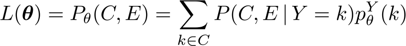
2.2 The likelihood

The likelihood to observe a subset C and an external information E can be expressed as

L (θ) = P_{θ} (C, E) = \sum_{k \in C} P (C, E ∣ Y = k) p_{θ}^{Y} (k)

The relation (1) allows us to relate p_k := P (C, E | Y = k) to $p_{k}^{*}$ and $q_{k}^{*}$ via

p_{k}^{*} = \frac{p_{k} q_{k}^{*}}{\sum_{l = 1}^{K} p_{l} q_{l}^{*}}

which is solved by

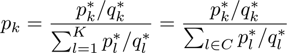
p_{k} = \frac{p_{k}^{*} / q_{k}^{*}}{\sum_{l = 1}^{K} p_{l}^{*} / q_{l}^{*}} = \frac{p_{k}^{*} / q_{k}^{*}}{\sum_{l \in C} p_{l}^{*} / q_{l}^{*}}

Consequently, we have

L (θ) = \sum_{k \in C} p_{k} p_{θ}^{Y} (k) = \frac{\sum_{k \in C} p_{k}^{*} / q_{k}^{*} p_{θ}^{Y} (k)}{\sum_{k \in C} p_{k}^{*} / q_{k}^{*}}

and this likelihood does not depend on E. Hence, its computation is feasible, even if E is not explicitly measured.

The classical CAR assumption can be expressed as

P (C, E | Y = k) does not depend on k for k \in C

This implies $p_{k}^{*} = q_{k}^{*} / \sum_{k \in C} q_{k}^{*}$ ; that is, the probability assigned to each possible value of k ∊ C is identical to the assumed distribution of Y conditioned on Y ∊ C. If we want to perform an analysis assuming CAR, we can choose arbitrary values for ${(q_{k}^{*})}_{k \in C}$ and choose $p_{k}^{*}$ accordingly.

The considerations above can be extended by accounting for additional variables X. We can replace p_θ (y) by a regression model, that is, by p_θ (y|x), or we can replace it by a multivariate distribution p_θ (y, x) with only the first variable affected by coarsening. In both situations, the prespecified probabilities $p_{k}^{*}$ and $q_{k}^{*}$ have to be interpreted as conditional probabilities given X. Details are outlined in appendix 2.

2.3 The scope of pccfit and pccprob

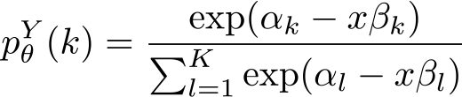
Because an explicit representation of the likelihood is available, we can use Stata’s ml command to obtain ML estimates of θ. This is exactly the purpose of pccfit. It assumes that the probabilities $p_{k}^{*}$ for each observation are represented in K variables and specifies the values $q_{k}^{*}$ as well as an expression for $p_{θ}^{Y} (k)$ . It also supports two standard choices of $p_{θ}^{Y} (k)$ . The first is a multinomial logistic regression model corresponding to Stata’s mlogit command. Here θ = (α ₁ ,…, α_K, β ₁ ,…, β_K ) and

p_{θ}^{Y} (k) = \frac{\exp (α_{k} - x β_{k})}{\sum_{l = 1}^{K} \exp (α_{l} - x β_{l})}

with α_b = 0 and β_b = 0 for one prespecified base outcome category b. This choice can be also used to fit simply a multinomial distribution by omitting any covariate. The second choice supports fitting regression models for ordered data. Here θ = (κ ₀ ,…, κ_K, β) and

p_{θ}^{Y} (k) = F (κ_{k} - x β) - F (κ_{k - 1} - x β)

with $κ_{0} = - \infty$ , $κ_{K} = \infty$ , and F denoting a prespecified distribution function. The choice F(y) = 1/{1+exp(−y)} corresponds to Stata’s ologit command, and the choice F = Φ to Stata’s oprobit command.

However, the presence of coarsened data already makes the estimation of the distribution of Y cumbersome. Hence, in many applications, the aim is not to fit regression models but just to obtain estimates of $P (Y = k) = p_{θ}^{Y} (k)$ Consequently, we also offer a postestimation command pccprob evaluating $p_{\hat{θ}}^{Y} (k)$ for any value k similar to Stata’s margins command.

2.4 A note of caution

We would like to point to one weakness of the ML approach: if there is a category with $p_{k}^{*} < 1$ for all observations but $p_{k}^{*} > 0$ 0 for some observations, it can nevertheless happen that the ML estimate $p_{\hat{θ}}^{Y} (k)$ equals 0. This is in particular problematic for many ordered categories because $p_{\hat{θ}}^{Y} (k)$ tends to lack smoothness. This can be avoided by specifying $p_{θ}^{Y} (k)$ as a smooth function of k. Consequently, we directly support the use of cubic splines in specifying $p_{θ}^{Y} (k)$ . However, the user can also simply specify other smooth functions, for example, polynomials.

3 The pccfit command

3.1 Syntax

The command expects to find K variables with the prespecified values p_k ^∗ for each observation. Categories outside C should have the value 0. The variables should share the same prefix with suffixes 1 to K. The syntax of pccfit is given by

pccfit [ indepvars ] [ if ] [ in] [ weight ], modelspecification numcat(integer)

[prefix(string) q(numlist | string) baseoutcome(integer) tolerance(real)

exact maximize_options]

The command fits the model specified by modelspecification to the data using the ML principle and the likelihood outlined in section 2.2. indepvars denotes potential covariates to be accounted for in the model specification. fweights, aweights, iweights, and pweights are allowed; they are passed to the ml command; see [U] 11.1.6 weight.

We now consider modelspecification. Here the user can explicitly define an expression for $p_{θ}^{Y} (k)$ (up to a normalizing constant) or refer to some prespecified models. The syntax is

modelspecification = usermodelspecification | prespecifiedmodelspecification

usermodelspecification = params( paramspecifications ) expr( exprspecification)

prespecifiedmodelspecification = mlogit| ologit| oprobit| odist( expr )

mlogit, ologit, and oprobit refer, respectively, to a multinomial logistic, ordered logistic, or ordered probit regression model. odist() refers to an ordered regression model with a user-specified choice of F. Here F is defined by expr with the argument of F denoted by a #. When the user specifies a model, params() defines the parameters in the parameter vector θ, and expr() defines an expression for $p_{θ}^{Y} (k)$ . The syntax of paramspecifications is

paramspecifications = paramspecification [| paramspecifications ]

paramspecification = {scalarpardef | vectorpardef }: [ varlist ] [,nocons ]

scalarpardef = name

vectorpardef = name numlist

In general, in the expression used to define $p_{θ}^{Y} (k)$ , you can refer to parameters by a name or by an indexed expression like alpha[3]. The first type of parameters is defined by a scalarpardef, and the second type of parameters, by a vectorpardef, with the numlist defining the index values to be considered. (Only nonnegative integers are allowed as indices, and they must appear in ascending order.) Parameters may actually refer to linear combinations of covariate vectors mimicking the equation specification in Stata’s ml command. This is specified by the : [ varlist ] [, nocons ] part. The varlist must be a subset of indepvars. For an example, see section 3.2.

exprspecification is a Stata expression that may include additional constructs evaluated in a preprocessing step for any possible value of k ∊ {1, 2,…, K}. After this preprocessing step, exprspecification should be a valid Stata expression if all (indexed) parameters are replaced by numbers.

The following additional constructs are allowed and evaluated during the preprocessing in the specified order:

{K} evaluates to K.

{k} evaluates to k.

{baseoutcome} evaluates to the value specified in the baseoutcome() option.

{cond( expr1 , expr2 , expr3 )} evaluates to expr2 if the evaluation of expr1 results in a value not equal to 0 and otherwise to expr3. expr2 and expr3 are preprocessed but not further evaluated as Stata expressions; that is, the preprocessed text of the selected expression replaces the {cond()} construct. Consequently, if the expressions include operators, it might be necessary to include the expression in parentheses to ensure correct interpretation. Note that the expressions may include further {cond()} constructs, which are evaluated prior to the preprocessing of the actual {cond()} construct.

{cubicspline( numlist , vectorpar , expr )} evaluates to an expression to compute a cubic spline function with knots at numlist and parameters according to vectorpar. The function is to be evaluated later at expr, but expr is not yet evaluated. vectorpar must be the name of a parameter vector with indices from 1 to the number of knots minus 1. vectorpar must have been specified accordingly in the params() option.

{ vectorpar [ expr ]} evaluates to vectorpar [ value ] with value denoting the value obtained from the evaluation of expr. vectorpar must have been specified as the name of a parameter vector in the params() option.

{ singlepar } evaluates to singlepar. singlepar must have been specified as the name of a single parameter in the params() option.

Note that the additional constructs described above do not allow additional spaces within the identifying parts of the different constructs, in particular, after a { and before a } sign.

Besides modelspecification, there is one additional option to be specified:

numcat( integer) defines the number of categories K. numcat() is required.

The following options can also be used:

prefix( string )defines the prefix of the variables used to store the values $p_{k}^{*}$ . By default, pccfit assumes that the variables are named p1,…, p K.

q( numlist | string ) specifies how the values $q_{k}^{*}$ are defined. If a numlist is given, it must be of length K, and it includes the values used for all observations. If no numlist is given, a single name is expected, and it is assumed that the values are specified for each observation in variables with a prefix equal to the specified name and numbered from 1 to K.

baseoutcome( integer ) defines a base outcome among the K categories, which can be referred to in modelspecification. By default, the most “frequent” category k is used, with the frequency defined by summing up the values of $p_{k}^{*}$ over all observations.

tolerance( real ) defines a tolerance for the deviation of the sum of the values $p_{k}^{*}$ or $q_{k}^{*}$ from 1.0. The default is tolerance(1.0e-5).

exact suppresses the computation of the normalizing constant and can be used if the expressions already define probabilities.

maximize_options are passed to the ml max command.

3.2 Methods and formulas

pccfit simply calls Stata’s ml function and applies it to the user-defined likelihood function using the lf evaluator. The likelihood function evaluates the expressions specified by the user for each single value of k ∊ {1, 2,…, K}. Then, $p_{θ}^{Y} (k)$ is computed by dividing each value by the sum of all values, that is, the normalizing constant. Finally, the likelihood for each observation is computed according to (2). Prior to these steps, each single parameter, singlepar, is replaced by the expression `singlepar’, and each indexed parameter vector, vectorpar [ value ], is replaced by `vectorpar value ‘ to match the arguments of the program used to evaluate the likelihood.

The mlogit option corresponds to the following usermodelspecification:

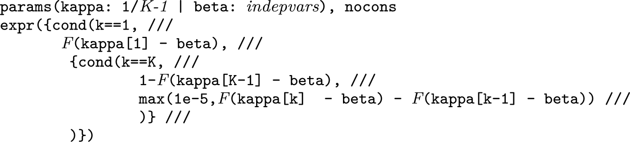
with the value of baseoutcome omitted in the numlist after alpha. The odist( expr ) option corresponds to the following usermodelspecification:

with F denoting the distribution function defined by expr. If pccfit is called without any independent variable, then the definition of beta and the term “- beta” is omitted. The ologit option corresponds to odist(logistic( # )) and oprobit to odist(normal( # )).

pccfit has the following side effects: an auxiliary program, pccmymodel, is needed by pccfit in calling ml. This is available as an additional ado-file and activated when executing pccfit.

3.3 Stored results

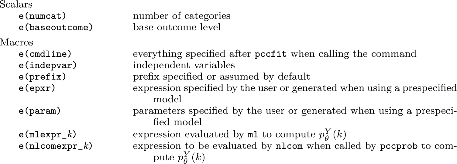
pccfit stores in e() the results generated by calling the ml command. In addition, it stores the following results:

4 The pccprob command

The pccprob command is a postestimation command to pccfit. It computes the probability P(Y ∊ S) for any subset S ⊂ {1, 2,…, K} according to the fitted model, that is, based on $p_{\hat{θ}}^{Y} (k)$ . The estimated probabilities are accompanied by standard errors and confidence intervals. The probabilities can be expressed on any transformation of the probability scale, and the results can be stored in e() or as a dataset, allowing one to use Stata’s graph commands for visualization. Several subsets can be handled simultaneously, supporting computation of cumulative and tail probabilities for ordered categories.

4.1 Syntax

The syntax of pccprob is given by

pccprob subsetspecifications [, trans( expr ) normaltrans( expr1 | expr2 )

post(normaltrans| nonormaltrans) nlcomoptions level( # ) label( valuelabel )

exact out add( addspec ) numlabel(min| max) outlabel( valuelabel )]

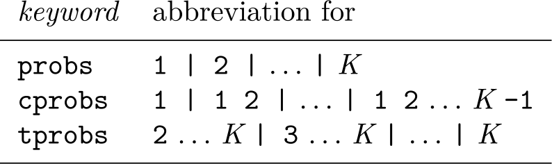
subsetspecifications is a sequence of numlists separated by | signs, and each numlist represents a subset of categories. Each numlist must be in ascending order. The sequence may also include the following keywords abbreviating sequences of numlists:

pccprob displays a table with the estimated probabilities, their standard errors, and confidence intervals. The probabilities are labeled by a list of numbers corresponding to the subsetspecification. The following options can be used to alter the output or to save the output:

trans( expr ) defines a transformation of the probability scale. expr can be any valid Stata expression with # denoting the argument.

normaltrans( expr1 | expr2 ) defines a transformation to be applied to the probabilities before computing confidence intervals. It should be chosen to get close to a normal distribution of the estimates. expr1 defines the transformation, expr2 the back transformation. In both expressions, # denotes the argument. If the trans() option is specified, the default is normaltrans(#|#); otherwise, the default is normaltrans(logit(#)|invlogit(#)).

post(normaltrans| nonormaltrans) posts estimation results in e(). normaltrans means that the estimates after the normalizing transformation are posted, and nonormaltrans means that the estimates as shown in the displayed output are posted. For naming of the estimates, the numlists defining the subsets are used but with all blanks removed and preceded by the suffix s.

nlcomoptions are passed to nlcom.

level( # ) sets the confidence level. The default is level(95).

label( valuelabel ) specifies a value label. This is applied to the values k ∊ {1, 2,…, K} in the output displayed. valuelabel must have been stored as a do-file with label save, with the label and the do-file having identical names.

exact suppresses including the normalizing constant in the computations of the probabilities and can be used if the expressions already define probabilities.

out saves the displayed table as the current Stata dataset. Hence, the dataset includes five variables: label, est, se, lb, and ub. The first variable is a string variable including the original label.

add( addspec ) adds one further observation to the dataset. addspec consists of numlist followed by an equal sign (=) and a number, indicating the label and the estimate to be added. No standard error or confidence intervals are added. add() requires that the option out be specified.

numlabel(min| max) replaces the label variable with a numerical variable including the minimal or the maximal category, respectively. numlabel() requires that the option out be specified.

outlabel( valuelabel ) specifies a value label added to the label variable if this is a numerical variable generated by using the numlabel() option. valuelabel must have been stored as a do-file with label save, with the label and the do-file having identical names. outlabel() requires that the option out be specified.

4.2 Methods and formulas

pccprob simply calls nlcom to compute the specified probabilities. The expressions for $p_{θ}^{Y} (k)$ suitable for the call of nlcom are already provided by pccfit. There is one basic difference to the expressions used by ml when executing pccfit: each parameter name parname is replaced by _b[ parname :_cons] or even by _b[ parname :_cons] + _b[ parname : var1 ] * var1 + · · · .

pccprob does not support an at option like the margin command. If you want to use pccprob after a model referring to covariates or other variables, you can define the variable values of interest as scalars and apply pccprob to an empty dataset. So a typical use looks like

If you want to include the set {1, 2,…, K} in the subsetspecification, you typically run into troubles because this set has the probability 1.0. For example, using the standard logit transformation to compute confidence intervals does not work. Thus, the numlist 1, 2,…, K is omitted when using the cprobs or tprobs keyword. You can use the add() option to add the corresponding value to the output dataset.

4.3 Stored results

As long as the post() option is not used, pccprob does not store any results.

4.4 A final note on the exact option

Both pccfit and pccprob offer the exact option, which can be used if the expressions specified in the expr() option do already define probabilities, such that there is no need to compute the normalizing constant. However, we do not recommend using this option with pccfit, because the normalizing constant contributes to the numerical stability of the computations. For example, ologit typically does not work when specifying exact, because the expressions used do not always define probabilities summing up exactly to 1.0. However, we recommend using this option when using pccprob because it avoids evaluating a long expression, which may even hit the maximally allowed expression length.

When you specify an expression corresponding to a multivariate distribution p_θ (y, x), you must specify the exact option in pccfit because otherwise the attempt to add a normalizing constant results in an incorrect likelihood. An example of this type can be found in section 5.3.

5 Examples

5.1 Example 1: Osteoarchaeological analysis

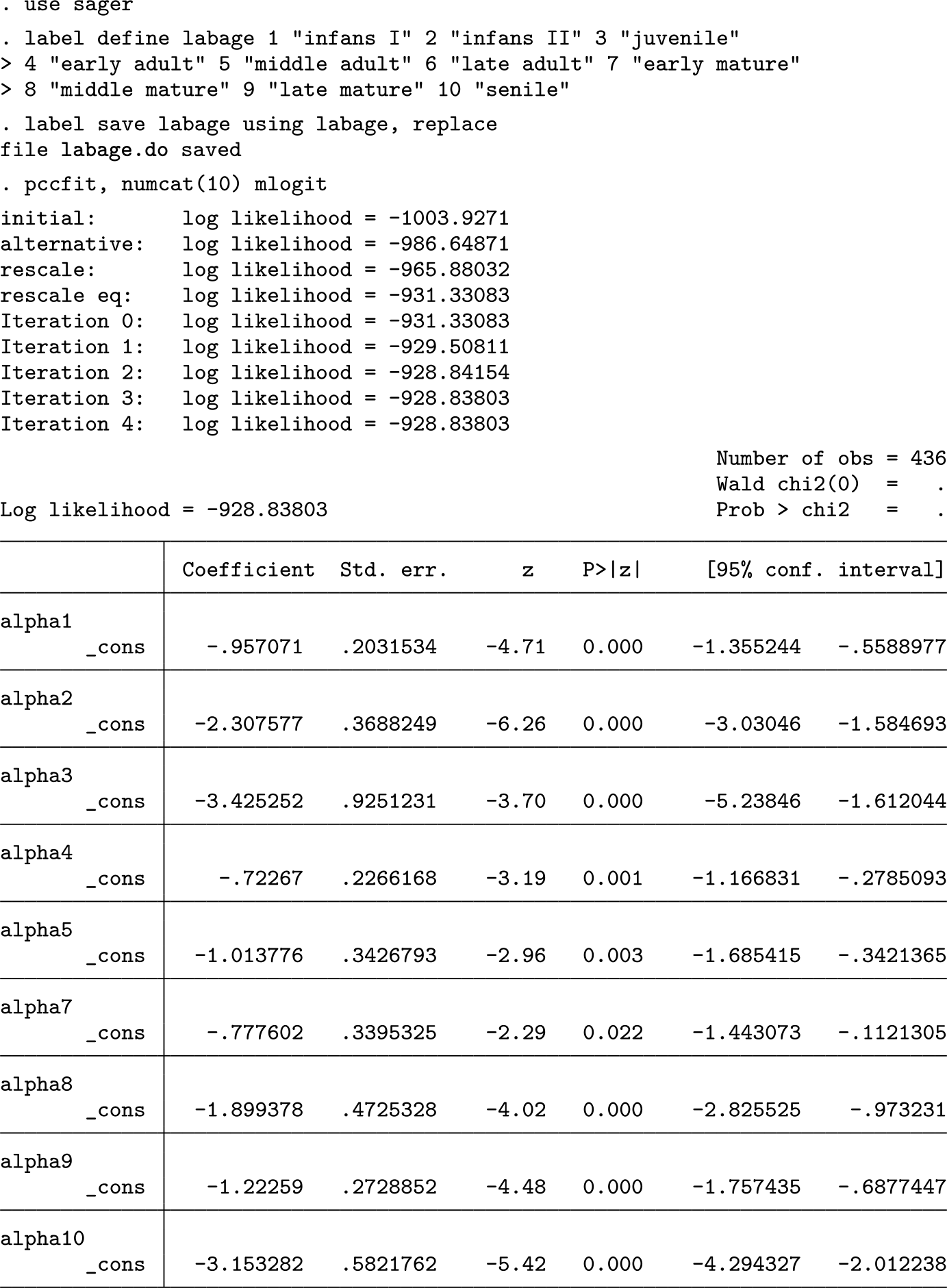
The Gallo–Roman burial site Im Sager is part of the Roman city of Augusta Raurica in northwest Switzerland (Berger 2012). The site comprises about 600 graves with inhumations and cremated skeletal remains of 436 individuals (Alder 2020). The burials were archaeologically and bioarchaeologically examined in an interdisciplinary study (Ammann Forthcoming). Determination of the age at death of the individuals buried at Im Sager is based on a system with the K = 10 categories infans I, infans II, juvenile, early adult, middle adult, late adult, early mature, middle mature, late adult, and senile (Großkopf 2004).

Only 81 subjects (18.6%) could be assigned to a single age class, and all other subjects could be assigned only to two or more classes. One hundred twenty-eight subjects (29.4%) were assigned to two classes, and 90 to three (20.6%). For 18 subjects (4.1%), it was impossible to exclude any class, and the remaining 119 subjects were assigned to 4 to 8 classes. On average, the age determination included 3.2 classes per individual. During the process of age determination, each possible class was labeled either as “more likely” or as “less likely” for each subject analyzed. These labels were transformed into probabilities by assigning the weights 1 and 2, respectively, and dividing the weight by the sum of weights within each subject. Among the 81 subjects assigned to a single class, 38 were classified as infans I, reflecting the straightforwardness of classifying young children. The age determination was performed by one assessor (Cornelia Alder), who made the decision between “less likely” or “more likely” solely based on the osteological findings without any assumptions on the underlying demographic distribution. This, together with the fact that each age class was assumed to have an age span of 7 years, justifies basing our analyses on the choice $q_{k}^{*} = 0.1$ .

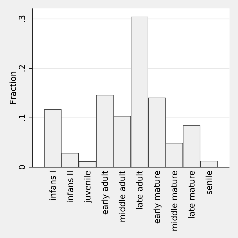
In a first step, we estimate the age distribution of the skeletal individuals and visualize this distribution as a bar chart mimicking a histogram. We obtain the following output and the graph shown in figure 1.

Figure 1.

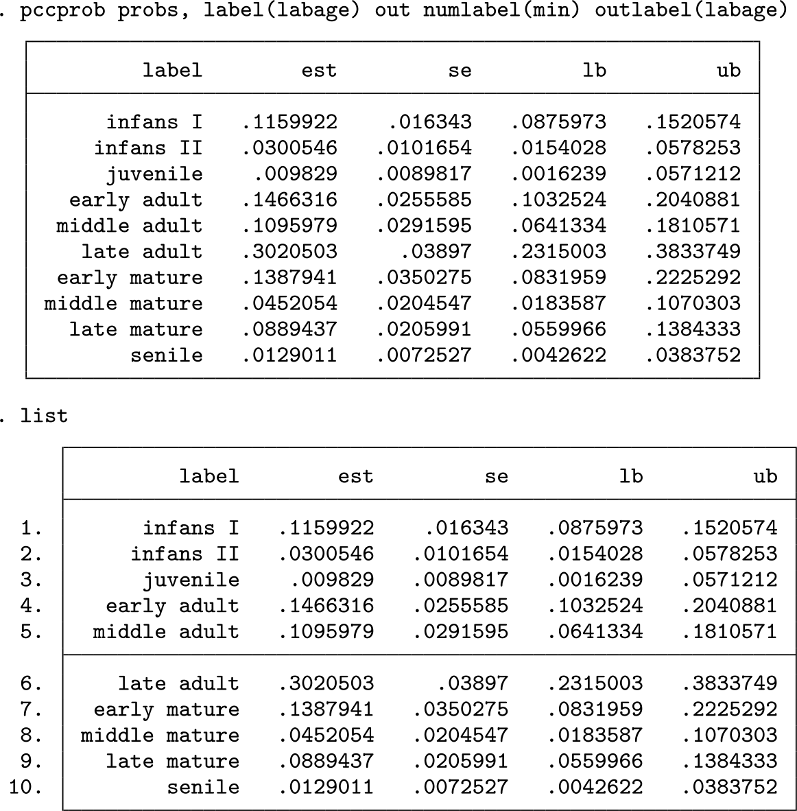
A histogramlike visualization of the estimated age distribution in example 1

We would like to point out that the confidence intervals for the single probabilities are rather wide. This is due to observing coarsened data, which carry less information than noncoarsened data. To illustrate this point, we compute the standard errors we would expect for noncoarsened data and consider the ratio of the observed standard errors to these standard errors:

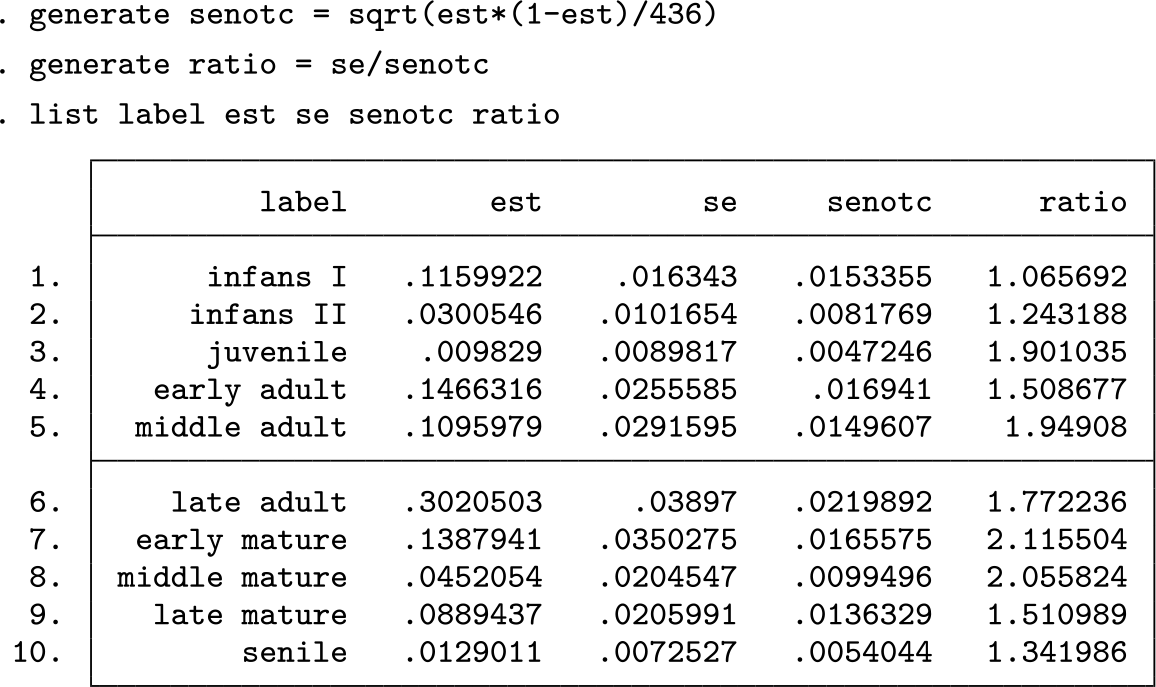
We observe standard errors inflated by a factor up to 2.1. The inflation is most pronounced for the middle-aged categories and least pronounced for infans I, infans II, and senile. This probably reflects the fact that individuals in these latter age groups are easier to determine because there are distinct indicators for either young or old, that is, high age. However, the gradual changes in trait morphology used to determine age in the “middle” categories lack distinctive cutoff markers, thus assigning individuals to many classes and increasing standard errors.

Consequently, we should be aware that the effective sample size is not 436 but probably less than 200. Any unreflected attempt to estimate the age distribution in 10 categories will hence suffer from limited precision, as reflected in rather wide confidence intervals. It might be more appropriate to visualize the age distribution by the cumulative distribution function because cumulative probabilities are less sensitive to coarsening. (To estimate the probability to be in a specific age category or above this category, any observation with a coarsened interval completely above or below this class contributes the same information as a subject with a noncoarsened observation.) We can approach this in the following way producing the graph shown in figure 2.

Figure 2.

The cumulative distribution function of the estimated age distribution in example 1

Using a parametric model for the class probabilities is another approach to obtain more stable estimates. We consider here a cubic spline with 5 knots equally spaced between 1.5 and 9.5. We can approach this by the following code producing the graph shown in figure 3.

Figure 3.

A histogramlike visualization of the estimated age distribution in example 1 based on using a cubic spline

We can now perform the same exercise as above and compare the standard errors with those to be expected frSom noncoarsened data and fitting a full multinomial model:

We observe ratios close to or below 1. This reflects that we estimate only four instead of nine parameters and that borrowing information from neighboring categories reduces the negative impact of coarsening.

Instead of estimating the full age distribution, we may focus on characteristics of the distribution like the mean. This can be approached by posting the estimates of the class probabilities and then building a weighted sum with weights, assigning to each age class the medium age according to the assumed span of seven years:

We can conclude that the average age at death in the skeletal population considered is about 34 years, with a rather small stochastic uncertainty visible in a narrow confidence interval.

The graves of the burial site Im Sager can be divided into two subgroups: inhumination and cremation burials. The burial practice may be related to the age at death of an individual; hence, it might be of interest to compare the age distribution between the two groups. The group of inhumination burials includes only 51 individuals; hence, we need to use a parametric model to come to stable estimates. We again use cubic splines and arrive at the graph shown in figure 4, indicating frequent use of inhumination in young children.

Figure 4.

Histogramlike visualizations of the estimated age distributions in cremation and inhumination burials in example 1 based on using a cubic spline

Finally, we may be interested in performing a formal significance test of the difference in age between the two groups. Because we may expect a shift in the age distribution— and the actually observed difference is also compatible with a shift—we can approach this using an ordered logistic regression model:

So the final conclusion is that we have a statistically significant difference in age between the two subpopulations with a p-value less than 0.0001, indicative of cultural processes affecting burial practices at Im Sager.

5.2 Example 2: Palaeodemographic analysis

So far, we have focused on analyzing the age distribution of the skeletal population. Palaeodemography goes one step further and attempts to make a link to the former living population the observed skeletal population originated from (Chamberlain 2006; Hoppa and Vaupel 2002a). When analyzing the skeletal population of a burial site associated with a settlement, we assume this to be the population living in the settlement and using the burial site for a certain period in time. The distribution of age at death among the deceased in the living population during the period the burial site was in use may be approximated by the age at death distribution in the skeletal population, if we can regard the latter as representative, that is, to be a random sample from the first. The validity of this assumption depends on many factors. It may be violated if some individuals died far from the settlement and were consequently not buried in the community where they had lived (for example, warriors or traders); if some of the deceased were buried elsewhere by cultural choice (for example, criminals or young children); or for taphonomic reasons, if, for example, age at death determined how deep graves were dug, thus affecting the preservation of childrens’ graves and skeletons (Knüsel and Robb 2016).

The next fundamental step is given by moving from the distribution of age at death to the age distribution among the living population and to age-specific mortality rates. Such quantities can be derived from the distribution of age at death, if we assume that the background population was stable in size and age composition over time (Coale 1972). This is a rather idealistic assumption (Sattenspiel and Harpending 1983) but nevertheless represents the basic assumption for demographic analysis of skeletal populations (Chamberlain 2006; Margerison and Knüsel 2002; Bonneuil 2005), which can give important insights into demographic side conditions for the society present in the settlement. The key step is that under these assumptions, the fraction of subjects at a certain age in the living population is equal to the fraction of subjects dying at this age or above this age when considering the distribution of age at death. So we can estimate the age distribution in the living population by computing the upper tail probabilities and rescaling them to probabilities, and we can then visualize them by a bar chart similar to a population pyramid (figure 5).

Figure 5.

Visualization of the estimated age distribution in the living population in example 2

Similarly, we can now compute mortality rates by comparing those dying while being in a certain age category with those dying at this age or above this age. The following piece of code generates a list of mortality rates for each age category together with a standard error:

We observe a very low mortality in the categories infans II and juvenile but an increased mortality rate in the category infans I, reflecting a well-known phenomenon. The mortality rates are about 15% in the first two adult age categories before we can see a substantial increase at higher age categories. The lack of a monotone trend suggests an instability that is not necessarily visible in the standard errors and suggests one perform some smoothing to obtain more reliable results. After such a postprocessing, the mortality rates can then be used to depict further aspects of mortality, for example, conditional survival probabilities or the life expectancy. Such computations are known as “life table analysis” (Halli and Rao 1992, chap. 2).

5.3 Example 3: A diagnostic accuracy study with an expert-based probabilistic reference standard

Here we consider an artificial dataset from a diagnostic accuracy study with a probabilistic reference standard based on an expert consensus. Not all subjects could be classified uniquely as diseased or undiseased; the experts assigned to some subjects a probability of 2/3 to be diseased and to some a probability of 1/3. Adding later the result of the index test to be evaluated in the variable test, we can use the following dataset for our analysis.

Category 1 refers to being undiseased (D = 0), and category 2 refers to being diseased (D = 1). Our interest is in sensitivity P (T = 1 | D = 1) and specificity P (T = 0 | D = 0).

The use of pccfit is now a little bit challenging. Sensitivity and specificity refer to the conditional distribution of T given D. However, the coarsened variable is D and not T. Hence, it is not sufficient to consider some model for T |D to be able to apply pccfit. One solution is to consider a model for the joint distribution of T and D. We can parameterize such a model via sensitivity, specificity, and the prevalence τ of D as

P (T = T, D = D) = {\begin{array}{l} {sens}^{T} (1 - {sens}^{(1 - T)} τ & if & D = 1 \\ {(1 - spec)}^{T} {spec}^{(1 - T)} (1 - τ) & if & D = 0 \end{array}

After transforming the three parameters from the probability to the logit scale, we can fit the model using pccfit. We cannot use pccprob to obtain the parameters of interest, but we can do this using nlcom as a postestimation command or—if we prefer more accurate confidence intervals based on a normal approximation on the logit scale—manually.

Because we have now used a multivariate model for the analysis, we have to ensure that the probabilities specified refer to the conditional probabilities of D given E and T. Of course, the experts were blinded to the index test T, and hence they definitely specified probabilities referring to D given E. We thus have to make here the additional assumption that the information in E was strong enough such that T would not have added additional information, if it had been known to the experts.

6 Discussion

6.1 Alternatives to ML estimation

6.1.1 Weighting

One simple alternative would be to interpret the specified probabilities p ^∗ just as weights. This means, for example, that we count a unit with $p_{1}^{*} = 0.5$ and $p_{2}^{*} = 0.5$ just as one half observation with Y = 1 and one half observation with Y = 2. With this approach, it would be simple to derive at an estimate for the distribution of Y : we just average the values of $p_{k}^{*}$ over all observations.

Unfortunately, this simple approach is just wrong and leads to biased results. To understand this, let us consider a simple example with two categories and a sample in which 80% of the observations fall in category 1 and 20% in category 2. We now introduce coarsened observations, and within these observations, the external information is so weak that we have to regard both categories as equally likely. This can be reflected by the choice $p_{k}^{*} = 0.5$ and $q_{k}^{*} = 0.5$ for k = 1, 2. We can randomly split our sample in two halves, one with observations of Y and one with coarsened observations. Because we do this randomly, we would expect that we are still able to recover the distribution of Y. However, if we apply the simple weighting approach, we will obtain estimates of about 65% and 35% because half the subjects contribute a weight of 0.5 and the other half on average a weight of 0.8 or 0.2, respectively. In contrast, the ML approach will arrive at correct estimates because in this simple situation, the ML approach will distribute the coarsened observations according to the distribution in the completely observed observations.

We can observe this issue also in our data, if we incorrectly apply the weighting approach. Figure 6 compares the result of the weighting approach with the ML approach. The rare categories are assigned a higher probability by the weighting approach than by the ML approach, and the frequent categories are assigned a lower probability. This flattening is in line with the considerations in the previous paragraph: The observations with high degree of coarsening are incorrectly flattened out over the whole range, whereas the ML approach avoids this and tries to distribute the coarsened data in line with the distribution observed in the less or noncoarsened observations.

Figure 6.

Visualization of the estimated age distribution in example 1 using the weighting approach or the ML approach

Nevertheless, the distinct peak for the category late adult in the distribution estimated by the ML approach is somewhat surprising. A closer look at the data in table 1, however, reveals that this reflects a true property of the dataset. We can observe that on one side the category late adult constitutes the category that is most rarely completely excluded. On the other side, it is also often assigned a probability of 1 (only exceeded by the category infans I) or a probability above 0.5 or at least above 1/3. Hence, in this dataset, some individuals could be assigned rather precisely to or close to this category, in spite of the gradual changes in trait morphology used to determine age in the “middle” categories mentioned above.

Table 1.

The distribution of the assigned probabilities p ^∗ for each age category in the total sample

	p ^∗
	0.0	$(0.0, \frac{1}{3}]$	$(\frac{1}{3}, \frac{1}{2}]$	$(\frac{1}{2}, 1.10)$	$1.10$
infans I	363	29	6	0	38
infans II	386	33	9	2	6
juvenile	363	51	21	0	1
early adult	272	112	42	8	2
middle adult	244	129	47	9	7
late adult	191	173	53	10	9
early mature	224	166	39	3	4
middle mature	259	156	17	0	4
late mature	284	126	16	3	7
senile	342	84	5	2	3

6.1.2 Bayesian inference

At first sight, the prespecified probabilities $p_{k}^{*}$ may look like a prior distribution of Y |C for a single observation. However, the choice of $p_{k}^{*}$ depends on the choice of $q_{k}^{*}$ and consequently, it seems to be more adequate to regard p_k —a function of all $p_{k}^{*}$ and $q_{k}^{*}$ —as prior probabilities. Assuming a flat, uninformative prior on θ, the posterior distribution is then proportional to L( θ ). The ML approach outlined in this article can hence also be seen as a computation of the mode of the posterior distribution. A full Bayesian approach can be implemented by allowing Y to be drawn from the values of C as part of a Markov chain Monte Carlo sampler.

6.1.3 Multiple imputation

Multiple imputation is another alternative to ML estimation. Luy and Wittwer-Backofen (2008) actually already considered a multiple imputation approach to obtain an estimate of the age distribution from coarsened age determination data without probabilistic information: for each coarsened observation of Y, they made a random draw from C (assuming a uniform distribution) and derived from this imputed dataset an estimate of the survival curve. And then they repeated this many times. However, this way to generate multiple imputations follows the spirit of the weighting approach, regarding the prespecified probabilities (constant within each C) as an estimate of the true distribution of Y. This is an example of an improper imputation method in the sense of Rubin (Rubin 1987; Nielsen 2003), resulting in biased estimates. Correct implementation of a multiple imputation approach would require one to develop a technique for generating proper multiple imputations.

6.1.4 Assuming CAR

Another approach would be to ignore the probabilistic information and to assume CAR. This can be a valid approach, too, because specifying probabilistic information does not necessarily imply that the CAR assumption is invalid. If the probabilistic information is based on measured additional external information, we just ignore this information, and hence become less efficient, but we do not necessarily introduce bias. However, the probabilistic information may also reflect an assumed violation of the CAR assumption. If we assume that one category implies more often a coarsening than another, we may account for this in the prespecification: We may tend to give this category a higher probability, even if otherwise several categories look equally likely.

6.2 Arriving at the probabilistic information

In both our examples, we considered the case that one or some subjects specify the probabilistic information. This is obviously a crucial step. One important aspect of this step is to make these subjects aware about the prior distribution of Y (reflected in the values $q_{k}^{*}$ ) they have in mind when specifying these probabilities. We may try to elicit this prior after the prespecification process has been finished or prior to this process. It is an open question which way is preferable. In the first case, we may fail to elicit this; in the second, we may raise unnecessary confusion.

6.3 Investigating the sensitivity to the specification of the probabilistic information

Because we may be in doubt about the validity of the prespecified probabilities, it seems reasonable to investigate the influence of these specifications on the results. One approach would be to ask different subjects to specify the probabilities and to compare the results. We may also add some noise to the probabilities and investigate the resulting fluctuation of the results. As pointed out above, we may also perform an analysis ignoring the probabilistic information and assuming CAR. In example 1, this approach results in the age distribution shown in figure 7, and this distribution is very similar to the one obtained when accounting for the probabilistic information (figure 1). So we can conclude that in this application, the prespecified probabilities have little influence on the final results.

Figure 7.

Visualization of the estimated age distribution in example 1 assuming CAR

6.4 Outlook

pccfit can be used to estimate the frequency distribution of a categorical variable with coarsened observations with or without additional probabilistic information or to include such variables as an outcome in a multinomial, ordered logistic, or ordered probit regression model. It hence adds useful functionality to Stata in handling such variables. It does not allow the use of such variables as an outcome in corresponding multilevel models, because here the likelihood is much harder to program. On the other side, the structure of the likelihood is very similar to the one covered by Stata’s gsem command. So future versions of gsem may also allow the handling of coarsened categorical outcome variables.

pccfit relies on ML as the statistical inference principle. As pointed out above, Bayesian inference may be considered as a basic alternative. A Bayesian approach may offer some advantages. For example, the computation of posterior distributions already requires some type of numerical integration, and hence it is often simple to integrate the additional summing about the unobserved values (because of coarsening) in the computational approach. Bayesian inference also avoids the problem of estimates on the boundary as described in section 2.4. Whereas the ML approach presented in this article considers many types of regression models with coarsened outcome data, the Bayesian approach may offer further flexibility with respect to handling missing covariate data, multilevel modeling, or adding temporal-spatial structures. The ML approach is also restricted to parametric smoothing approaches such as splines, whereas Bayesian inference integrates more general smoothing approaches. However, the use of the Bayesian approach requires to clarify the role of the prespecified probabilities $p_{k}^{*}$ within a Bayesian framework.

Human osteoarchaeology is a field where coarsened data with or without probabilistic information occurs as a matter of fact. In osteological sex determination, the traditional approach was to develop rules assigning sex on a 3-point-scale (f, ?, m) or a 5-point scale (f, f?, ?, m?, m), that is, in a specific way to code probabilistic information on the binary variable sex. However, this is now changing by publishing rules allowing computation of posterior probabilities (Brůžek et al. 2017), that is, exact probabilistic information. The Rostock manifesto has emphasized the need of using posterior probabilities not only for sex but also for anthropological age determination (Hoppa and Vaupel 2002b).

In the field of archaeology, in general, coarsened data appear in the context of working with chronological orders. For many features of objects, it is known how to map them to a certain time span, and even within this time span, frequency differences are known, resulting in probabilistic information. The mathematical procedure to develop such mappings, known as “seriation” was developed by Sir William Flinders Petri as early as the end of the 19th century (Renfrew and Bahn 2019), and today many such chronologies are available.

We considered an expert-based reference standard as a further example for coarsened data. The emphasis on prediction in the upcoming field of data sciences will probably generate many prediction models in the future, which then will be applied to generate input in further applications. In all of these cases, we will be forced to work with coarsened data with probabilistic information.

7 Programs and supplemental materials

Supplemental Material, sj-zip-1-stj-10.1177_1536867X221083902 - Analyzing coarsened categorical data with or without probabilistic information

Supplemental Material, sj-zip-1-stj-10.1177_1536867X221083902 for Analyzing coarsened categorical data with or without probabilistic information by Werner Vach, Cornelia Alder and Sandra Pichler in The Stata Journal

Footnotes

7 Programs and supplemental materials

To install a snapshot of the corresponding software files as they existed at the time of publication of this article, type

Appendix 1: Choice of q k * in the case of using a predefined prediction rule

We consider now the specific situation of a binary outcome Y, C = {0, 1} always and E = X representing measured covariates. The probabilities $p_{1}^{*}$ are based on a prediction rule, providing estimates of P (Y = 1|X = x) developed in an external population. We are typically not much aware about the influence of the population prevalence of Y (that is, of its marginal distribution) on such a prediction rule, because we are directly modeling the conditional distribution of Y given X. However, there is still such a relation, because

This suggests that we should choose q ₁ ^∗ as the prevalence of Y in the external population. This is a safe choice, if a potential difference in the prevalence between the external population and the current study population can be explained by a selection in dependence on Y. In this case, we know that P (X|Y ) is identical in the two populations, which is the assumption we make in deriving the likelihood in section 2.2, if the values p ₁ ^∗ are derived from an external population. However, if there is a selection in dependence on X, the situation is more complicated because P (X|Y ) will change, too. However, the relation (1) may still hold approximately because P(X|Y = 1) and P (X|Y = 0) are affected similarly. This question requires further investigation.

Appendix 2: Accounting for additional variables X

In the case of interest in a model p_θ (y|x), the likelihood of interest is

The values $p_{k}^{*}$ and $q_{k}^{*}$ now refer to the conditional probabilities P (Y = k | C, E, X) and P (Y = k | X) and reflect the implicit knowledge about the conditional coarsening mechanism and the conditional distribution of E given Y and X. The relation (1) now reads

and connects the prespecified probabilities to the likelihood.

In the case of interest in a multivariate model p_θ (y, x), the likelihood of interest is

and exactly the same arguments can be applied.

References

Alder

. 2020. “Dem Ritus auf der Spur”, Anthropologische Auswertung des Gräberfeldes Im Sager von Augusta Raurica/Schweiz.

Ammann

. Forthcoming. Das Südostgräberfeld von Augusta Raurica. Archäologische und naturwissenschaftliche Untersuchungen im römerzeitlichen Gräberfeld Im Sager, Kaiseraugst/AG. (mit naturwissenschaftlichen Beiträgen von Sabine Deschler-Erb, Örni Akeret, Angela Schlumbaum, Christine Prümpin und Philippe Rentzel sowie Fundauswertungsbeiträgen von Sylvia Fünfschilling, Ruedi Kaenel und Markus Peter).

Berger

2012. Führer durch Augusta Raurica. Basel: Schwabe Verlag.

Bonneuil

2005. Fitting to a distribution of deaths by age with application to paleodemography: The route closest to a stable population. Current Anthropology 46: S29–S45. https://doi.org/10.1086/444367.

Brůžek

Santos

Dutailly

Murail

Cunha

2017. Validation and reliability of the sex estimation of the human os coxae using freely available DSP2 software for bioarchaeology and forensic anthropology. American Journal of Physical Anthropology 164: 440–449. https://doi.org/10.1002/ajpa.23282.

Chamberlain

. 2006. Demography in Archaeology. Cambridge: Cambridge University Press. https://doi.org/10.1017/CBO9780511607165.

Coale

A. J.

1972. Growth and Structure of Human Populations: A Mathematical Investigation. Princeton, NJ: Princeton University Press.

Gill

R. D.

van der Laan

M. J.

Robins

J. M.

1997. Coarsening at random: Characterizations, conjectures, counter-examples. In Proceedings of the First Seattle Symposium in Biostatistics, ed. Lin

D. Y.

Fleming

T. R.

, 255–294. New York: Springer. https://doi.org/10.1007/978-1-4684-6316-3_14.

Großkopf

2004. Leichenbrand. Biologisches und kulturhistorisches Quellenmaterial zur Rekonstruktion vorund frühgeschichtlicher Populationen und ihrer Funeralpraktiken. PhD thesis, University of Leipzig.

10.

Halli

S. S.

Rao

K. V.

1992. Advanced Techniques of Population Analysis. Boston: Springer. https://doi.org/10.1007/978-1-4757-9030-6.

11.

Heitjan

D. F.

Rubin

D. B.

1991. Ignorability and coarse data. Annals of Statistics 19: 2244–2253. https://doi.org/10.1214/aos/1176348396.

12.

Hoppa

R. D.

Vaupel

J. W.

, eds. 2002a. Paleodemography: Age Distributions from Skeletal Samples. Cambridge: Cambridge University Press.

13.

Hoppa

R. D.

Vaupel

J. W.

2002b. The Rostock Manifesto for paleodemography: The way from stage to age. In Paleodemography: Age Distributions from Skeletal Samples, ed. Hoppa

R. D.

Vaupel

J. W.

, 1–8. Cambridge: Cambridge University Press. https://doi.org/10.1017/CBO9780511542428.001.

14.

Jenniskens

Naaktgeboren

C. A.

Reitsma

J. B.

Hooft

Moons

K. G.

van Smeden

2019. Forcing dichotomous disease classification from reference standards leads to bias in diagnostic accuracy estimates: A simulation study. Journal of Clinical Epidemiology 111: 1–10. https://doi.org/10.1016/j.jclinepi.2019.03.002.

15.

Knüsel

C. J.

Robb

2016. Funerary taphonomy: An overview of goals and methods. Journal of Archaeological Science: Reports 10: 655–673. https://doi.org/10.1016/j.jasrep.2016.05.031.

16.

Luy

M. A.

Wittwer-Backofen

2008. The Halley band for paleodemographic mortality analysis. In Recent Advances in Palaeodemography: Data, Techniques, Patterns, ed. Bocquet-Appel

J.-P.

, 119–141. Dordrecht: Springer. https://doi.org/10.1007/978-1-4020-6424-1_5.

17.

Margerison

B. J.

Knüsel

C. J.

2002. Paleodemographic comparison of a catastrophic and an attritional death assemblage. American Journal of Physical Anthropology 119: 134–143. https://doi.org/10.1002/ajpa.10082.

18.

Nielsen

S. F.

2003. Proper and improper multiple imputation. International Statistical Review 71: 593–607. https://doi.org/10.1111/j.1751-5823.2003.tb00214.x.

19.

Renfrew

Bahn

2019. Archaeology: Theories, Methods and Practice. 8th ed. London: Thames & Hudson.

20.

Rubin

D. B

. 1987. Multiple Imputation for Nonresponse in Surveys. New York: Wiley. https://doi.org/10.1002/9780470316696.

21.

Sattenspiel

Harpending

1983. Stable populations and skeletal age. American Antiquity 48: 489–498. https://doi.org/10.2307/280557.

22.

White

T. D.

Black

M. T.

Folkens

P. A.

2011. Human Osteology. 3rd ed. Burlington, MA: Academic Press. https://doi.org/10.1016/C2009-0-03221-8.

Supplementary Material

Please find the following supplemental material available below.

For Open Access articles published under a Creative Commons License, all supplemental material carries the same license as the article it is associated with.

For non-Open Access articles published, all supplemental material carries a non-exclusive license, and permission requests for re-use of supplemental material or any part of supplemental material shall be sent directly to the copyright owner as specified in the copyright notice associated with the article.

0.01 MB

0.00 MB