Measuring technical efficiency and total factor productivity change with undesirable outputs in Stata

Abstract

In this article, we introduce two community-contributed data envelopment analysis commands for measuring technical efficiency and productivity change in Stata. Over the last decades, an important theoretical progression of data envelopment analysis, a nonparametric method widely used to assess the performance of decision-making units, is the incorporation of undesirable outputs. Models able to deal with undesirable outputs have been developed and applied in empirical studies for assessing the sustainability of decision-making units. These models are getting more and more attention from researchers and managers. The teddf command discussed in the present article allows users to measure technical efficiency, both radial and nonradial, when some outputs are undesirable. Technical efficiency measures are obtained by solving linear programming problems. The gtfpch command we also describe here provides tools for measuring productivity change, for example, the Malmquist–Luenberger index and the Luenberger indicator. We provide a brief overview of the nonparametric efficiency and productivity change measurement accounting for undesirable outputs, and we describe the syntax and options of the new commands. We also illustrate with examples how to perform the technical efficiency and productivity analysis with the newly introduced commands.

1 Introduction

After the pioneering work of Farrell (1957), Debreu (1951), and Koopmans (1951), efficiency and productivity analysis have been widely used in empirical studies to assess the performance of decision-making units (dmus) in terms of converting inputs into outputs. Among the parametric and nonparametric frontier models that have been developed in the field of efficiency analysis, data envelopment analysis (dea) has received plenty of attention because it does not need prior information of the production function form and because of its capability in multiple output technologies (Färe, Grosskopf, and Lovell 1985; Färe et al. 1994). Efficiency analysis based on dea usually assumes that inputs should be shrunk and outputs should be expanded. However, in the real world, outputs are not always desirable. In the case of undesirable outputs, they should be shrunk to improve efficiency.

With the increasing demand in the last decades to improve the sustainability of the economic society, scholars and managers have recognized that it is vital to consider undesirable output in efficiency and productivity analysis (Chung, Färe, and Grosskopf 1997; Mahlberg and Sahoo 2011). Correspondingly, dea models able to deal with undesirable outputs have been developed and applied in empirical studies, for example, Zhou, Ang, and Wang (2012) and Lin and Du (2015).

The estimation of nonparametric frontier models can be readily performed in Stata with some community-contributed commands. The dea command proposed in Ji and Lee (2010) provides a basic tool to estimate radial technical efficiency using the dea technique in Stata. Badunenko and Mozharovskyi (2016) extended dea with five new commands that allow users to implement both radial and nonradial technical efficiency estimation, as well as statistical inference in nonparametric frontier models in Stata. Tauchmann (2012) introduced two commands, orderm and orderalpha, for implementing order-m, order-α, and free disposal hull efficiency analysis in Stata. All these commands, however, are limited in their capability to perform efficiency and productivity analysis with undesirable outputs.

Here we introduce two community-contributed commands for measuring technical efficiency and productivity change with undesirable outputs in Stata. teddf estimates the directional distance function (ddf) with undesirable outputs for technical efficiency measurement. Both radial Debreu–Farrell and nonradial Russell measures can be calculated under different assumptions about the production technology, for example, window, biennial, sequential, and global production technology. gtfpch measures the total factor productivity (tfp) change with undesirable outputs by using the Malmquist– Luenberger productivity index (mlpi) or the Luenberger indicator. The new commands make it effortless to perform efficiency and productivity analysis with undesirable outputs in Stata, and their results can directly feed to other commands for further analysis.

The remainder of this article unfolds as follows: section 2 provides a brief overview of the nonparametric efficiency and productivity change measurement while accounting for undesirable outputs; sections 3 and 4 explain the syntax and options of teddf and gtfpch, respectively; section 5 presents a hypothetical example to illustrate usage of the two commands; and section 6 concludes the article.

2 The model

In this section, we provide a brief overview of the nonparametric efficiency and productivity measurement accounting for undesirable outputs. The radial and nonradial ddf will be introduced, followed by a description of the measurement of technical efficiency and tfp change using ddfs. The exposition here is only introductory. For more details, please refer to the cited works.

2.1 DDF

Consider a production unit transforming a vector of nonnegative inputs into a vector of nonnegative desirable outputs and a vector of by-products (undesirable outputs), such as pollution, subject to the constraint imposed by a fixed technology. For the production technology, inputs and desirable outputs are supposed to be strongly disposable. The undesirable outputs are assumed to be weakly disposable, which indicates that the decrease of undesirable outputs is not free but will lead to a deduction in desirable outputs. If we denote the inputs, desirable outputs, and undesirable outputs as $x\in {\Re }_{+}^N$ , $y\in {\Re }_{+}^M$ , and $b\in {\Re }_{+}^H$ , respectively, then the production technology described above can be characterized by the technology set as

$T=\{(\mathit{x},\mathit{y},\mathit{b}):\mathit{x}\text{can produce }(\mathit{y},\mathit{b})\}$

Then, following Chung, Färe, and Grosskopf (1997), the radial ddf is defined as

$D_r(\mathit{x},\mathit{y},\mathit{b};\mathit{g}) =\text{sup}[\beta :\{(\mathit{x},\mathit{y},\mathit{b})+\beta \mathit{g}\}\in T]$

1

where $\mathit{g}=({\mathit{g}}_{\mathit{x}},{\mathit{g}}_{\mathit{y}},{\mathit{g}}_{\mathit{b}})\in \hspace{0.17em}{\Re }_{-}^N\times {\Re }_{+}^M\times {\Re }_{-}^H$ is a preassigned nonzero vector specifying the direction in which the distance between the data point, ( x , y, b ), and the production frontier is measured.

Equation (1) gives the most general form of radial ddf. One can define the distance between the dmu and the production frontier in a specific direction by setting different g . To illustrate, we consider the cases of g ₁ = (0 , y, 0), g ₂ = (0, 0 , − b ), and g ₃ = (0 , y, − b ), which are widely used in literature. Figure 1 presents hypothetical production processes with one desirable output (for example, gross domestic product) and one undesirable output (for example, CO₂). Conceptually, in figure 1, $\overline{A\mathit{b}}$ and $\overline{AC}$ represent the distance when the direction is g ₁ = (0 , y, 0) and g ₂ = (0, 0 , − b ), respectively. The former focuses on economic prosperity, while the latter focuses on environmental protection. Similarly, $\overline{AD}$ is the distance when the direction is g ₃ = (0 , y, − b ), which describes the maximum increase of desirable output while simultaneously reducing the undesirable output along the direction ( y , − b ). Intuitively, the smaller the distance, the closer the dmu is to the production frontier (the distance is 0 for a dmu that operates on the production frontier).

Figure 1.

A graphical illustration of ddfs

The radial measure expands (shrinks) all outputs and inputs proportionally until the production frontier is reached. At the reached frontier point, some but not all outputs (inputs) can be expanded (shrunk) while remaining feasible. If such a possibility is available for a given dmu for some outputs (inputs), then the reference point is said to have slacks in outputs (inputs). Nonradial measures, that is, the Russell measure, accommodate such slacks (Chambers 2002; Färe and Grosskopf 2010; Zhou, Ang, and Wang 2012).

The nonradial ddf is defined as

$D_{nr}(\mathit{x},\mathit{y},\mathit{b};\mathit{g})=\sup \left[w\beta :\{(\mathit{x},\mathit{y},\mathit{b})+\mathrm{diag}(\beta )\times \mathit{g}\}\in T\right]$

where w denotes a nonnegative weight vector; β = ( β _x,β _y,β _b ) ∊ ℜ ^N × ℜ ^M × ℜ ^H , where β_x , β_y , and β_b denote the vectors of the scaling factors with regard to inputs ( x ), desirable outputs ( y ), and undesirable outputs ( b ), respectively. Clearly, the nonradial ddf measure allows the inputs and outputs to be adjusted nonproportionally. The reference point in a nonradial ddf can be located at any point on the production frontier (in contrast to the radial measure in figure 1, where the reference point is a fixed point, such as B, C, or D).

2.2 Measurement of technical efficiency

To estimate the ddf measure of technical efficiency using the nonparametric technique, the production technology set is derived from observed data. Typically, for crosssectional data with J individuals, the production technology set with the assumption of constant returns to scale (crs) is constructed as

$T=\left\{(\mathit{x},\mathit{y},\mathit{b}):{\displaystyle \sum _{j=1}^J{\lambda }_j}{\mathit{x}}_j\le \mathit{x},{\displaystyle \sum _{j=1}^J{\lambda }_j}{\mathit{y}}_j\ge \mathit{y},{\displaystyle \sum _{j=1}^J{\lambda }_j}{\mathit{b}}_j=\mathit{b},\hspace{0.17em}\lambda \ge 0\right\}$

For variable returns to scale (vrs), ${\displaystyle \sum { }_{j=1}^J}\hspace{0.17em}{\lambda }_j\hspace{0.17em}=\hspace{0.17em}1$ is added to the above equation. That is,

$T=\left\{(\mathit{x},\mathit{y},\mathit{b}):{\displaystyle \sum _{j=1}^J{\lambda }_j}{\mathit{x}}_j\le \mathit{x},{\displaystyle \sum _{j=1}^J{\lambda }_j}{\mathit{y}}_j\ge \mathit{y},{\displaystyle \sum _{j=1}^J{\lambda }_j}{\mathit{b}}_j=\mathit{b},\lambda \ge 0,{\displaystyle \sum _{j=1}^J{\lambda }_j}=1\right\}$

In the panel-data context, the time-series dimension can provide more information on the production technology. Researchers have proposed different types of production technology sets, such as global, sequential, window, biennial, and contemporaneous production technology. The production technology set at time t is as follows:

$\begin{array}{l}T(t)=\\ \left\{(\mathit{x},\mathit{y},\mathit{b}):{\displaystyle \sum _{\tau \in {\Gamma }_t}{\displaystyle \sum _{j=1}^J{\lambda }_{j\tau }}}{\mathit{x}}_{j\tau }\le \mathit{x},{\displaystyle \sum _{\tau \in {\Gamma }_t}{\displaystyle \sum _{j=1}^J{\lambda }_{j\tau }}}{\mathit{y}}_{j\tau }\ge \mathit{y},{\displaystyle \sum _{\tau \in {\Gamma }_t}{\displaystyle \sum _{j=1}^J{\lambda }_{j\tau }}}{\mathit{b}}_{j\tau }=\mathit{b},\hspace{0.17em}\lambda \ge 0\right\}\end{array}$

The time range, τ ∊ Γ _t , for different types of production technology sets are shown in figure 2. In the global production technology, τ ∊ Γ _t is expressed as τ ≤ t _max, where t _max is the last period in the sample. In the sequential production technology, τ ∊ Γ _t is expressed as τ ≤ t. In the window production technology, τ ∊ Γ _t is expressed as t − h ≤ τ ≤ t + h, where h is the bandwidth. In the biennial production technology, τ ∊ Γ _t is expressed as t ≤ τ ≤ t + 1. In the contemporaneous production technology, τ ∊ Γ _t is expressed as τ = t.

Figure 2.

Timing assumptions of different types of production technology sets

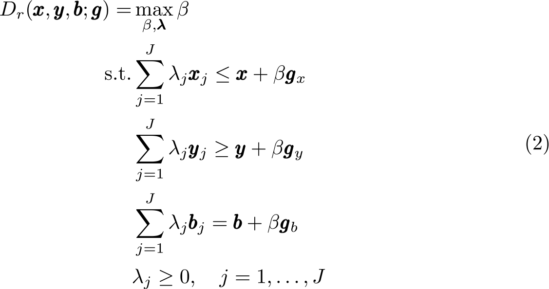
Then the radial ddf measure of inefficiency under the crs assumption can be estimated by solving the following linear programming problem:

$\begin{array}{l}{D}_r(\mathit{x},\mathit{y},\mathit{b};\mathit{g})=\underset{\beta ,\lambda }{\max }\beta \\ \text{s.t. }{\displaystyle \sum _{j=1}^J{\lambda }_j}{\mathit{x}}_j\le \mathit{x}+\beta {\mathit{g}}_{\mathit{x}}\\ {\displaystyle \sum _{j=1}^J{\lambda }_j}{\mathit{y}}_j\ge \mathit{y}+\beta {\mathit{g}}_{\mathit{y}}\\ {\displaystyle \sum _{j=1}^J{\lambda }_j}{\mathit{b}}_j=\mathit{b}+\beta {\mathit{g}}_{\mathit{b}}\\ {\lambda }_j\ge 0,j=1,\dots ,J\end{array}$

2

This technology set is based on the assumption of crs. For a vrs assumption, ${\displaystyle \sum { }_{j=1}^J}\hspace{0.17em}{\lambda }_j\hspace{0.17em}=\hspace{0.17em}1$ is added to the above constraints.

In (2), the left-hand side of the constraints construct the production frontier using the convex hull of the observation data. The right-hand side allows the assessed dmu to adjust the inputs ( x ), the desirable outputs ( y ), and the undesirable outputs ( b ) along the direction of ( g _x,g _y,g _b ). The ddf seeks to maximize the reduction of inputs and undesirable outputs and the expansion of the desirable output in means of ( x +β g _x,y + β g _y,b + β g _b ) given the production technology.

Similarly, the nonradial ddf measure of inefficiency accounting for the undesirable outputs can be obtained by solving the following linear programming problem:

$\begin{array}{l}{D}_{nr}(\mathit{x},\mathit{y},\mathit{b};\mathit{g})=\underset{\beta ,\lambda }{\max }{w}^{\prime }\beta \\ \hspace{0.17em}\text{s.t. }{\displaystyle \sum _{j=1}^J{\lambda }_j}{\mathit{x}}_j\le \mathit{x}+\mathrm{diag}\left({\beta }_{\mathit{x}}\right)\times {\mathit{g}}_{\mathit{x}}\\ \hspace{0.17em}{\displaystyle \sum _{j=1}^J{\lambda }_j}{\mathit{y}}_j\ge \mathit{y}+\mathrm{diag}\left({\beta }_{\mathit{y}}\right)\times {\mathit{g}}_{\mathit{y}}\\ \hspace{0.17em}{\displaystyle \sum _{j=1}^J{\lambda }_j}{\mathit{b}}_j=\mathit{b}+\mathrm{diag}\left({\beta }_{\mathit{b}}\right)\times {\mathit{g}}_{\mathit{b}}\\ \hspace{0.17em}\beta \ge 0;{\lambda }_j\ge 0,j=1,\dots ,J\end{array}$

For a vrs assumption, ${\displaystyle {\sum }_{j=1}^J{\lambda }_j\hspace{0.17em}=\hspace{0.17em}1}$ is added to the above constraints.

Unlike the ddf shown in (2), the nonradial ddf allows each component of inputs, desirable outputs, and undesirable outputs to adjust in varying proportions. The nonradial ddf is the maximum weighted sum of the adjustment components (β) such that [diag(β_x ) × g _x, diag(β_y ) × g _y, diag(β_b ) × g _b ] can be produced given the production technology.

For the panel-data case, the radial ddf measure of inefficiency under the crs assumption can be estimated by solving the following linear programming problem:

$\begin{array}{l}{D}_r(\mathit{x},\mathit{y},\mathit{b};\mathit{g})=\underset{\beta ,\lambda }{\max }\beta \\ \text{s.t. }{\displaystyle \sum _{\tau \in {\Gamma }_t}{\displaystyle \sum _{j=1}^J{\lambda }_{j\tau }}}{\mathit{x}}_{j\tau }\le \mathit{x}+\beta {\mathit{g}}_{\mathit{x}}\\ {\displaystyle \sum _{\tau \in {\Gamma }_t}{\displaystyle \sum _{j=1}^J{\lambda }_{j\tau }}}{\mathit{y}}_{j\tau }\ge \mathit{y}+\beta {\mathit{g}}_{\mathit{y}}\\ {\displaystyle \sum _{\tau \in {\Gamma }_t}{\displaystyle \sum _{j=1}^J{\lambda }_{j\tau }}}{\mathit{b}}_{j\tau }=\mathit{b}+\beta {\mathit{g}}_{\mathit{b}}\\ {\lambda }_{j\tau }\ge 0,j=1,\dots ,J\end{array}$

Similarly, for the panel-data case, the nonradial ddf measure of inefficiency can be estimated by solving the following linear programming problem:

$\begin{array}{l}{D}_r(\mathit{x},\mathit{y},\mathit{b};\mathit{g})=\underset{\beta ,\lambda }{ma\mathit{x}} w^{\prime }\beta \\ \text{s.t. }{\displaystyle \sum _{\tau \in {\Gamma }_t}{\displaystyle \sum _{j=1}^J{\lambda }_{j\tau }}}{\mathit{x}}_{j\tau }\le \mathit{x}+\mathrm{diag}\left({\beta }_{\mathit{x}}\right)\times {\mathit{g}}_{\mathit{x}}\\ {\displaystyle \sum _{\tau \in {\Gamma }_t}{\displaystyle \sum _{j=1}^J{\lambda }_{j\tau }}}{\mathit{y}}_{j\tau }\ge \mathit{y}+\mathrm{diag}\left({\beta }_{\mathit{y}}\right)\times {\mathit{g}}_{\mathit{y}}\\ {\displaystyle \sum _{\tau \in {\Gamma }_t}{\displaystyle \sum _{j=1}^J{\lambda }_{j\tau }}}{\mathit{b}}_{j\tau }=\mathit{b}+\mathrm{diag}\left({\beta }_{\mathit{b}}\right)\times {\mathit{g}}_{\mathit{b}}\\ \beta \ge 0;{\lambda }_{j\tau }\ge 0,j=1,\dots ,J\end{array}$

2.3 Measurement of TFP change

The measurement of productivity change has traditionally focused on measuring marketable (desirable) outputs of dmus relative to paid factors of production. This approach, which typically ignores the production of by-products such as pollution, can yield biased measures of productivity growth (Chung, Färe, and Grosskopf 1997). For example, firms in industries that face environmental regulations would typically find that their productivity is adversely affected, because the costs of abatement capital would typically be included on the input side but no account would be made of the reduction in pollutants on the output side.

Chung, Färe, and Grosskopf (1997) introduced a productivity index based on the radial ddf measure, called the mlpi, which credits the reduction of undesirable outputs— for example, pollution—while simultaneously crediting increases in desirable outputs. Consider two adjacent periods, denoted as s and t, respectively. If we choose the direction to be g = (0 ,y, − b ), then the output-oriented mlpi with undesirable outputs is defined as

$\text{ML}={\left\{\frac{1+D_r^t\left({\mathit{x}}^s,{\mathit{y}}^s,{\mathit{b}}^s;\mathit{g}\right)}{1+D_r^t\left({\mathit{x}}^t,{\mathit{y}}^t,{\mathit{b}}^t;\mathit{g}\right)}\times \frac{1+D_r^s\left({\mathit{x}}^s,{\mathit{y}}^s,{\mathit{b}}^s;\mathit{g}\right)}{1+D_r^s\left({\mathit{x}}^t,{\mathit{y}}^t,{\mathit{b}}^t;\mathit{g}\right)}\right\}}^{1/2}$

To avoid an arbitrary choice between base years, a geometric mean of a fractionbased mlpi in base year t (first fraction) and s (second fraction) has been taken. The Malmquist–Luenberger measure indicates productivity improvement if the value is greater than 1 and indicates a decrease in productivity if the value is less than 1.

The mlpi can be decomposed into two components (Chung, Färe, and Grosskopf 1997), one accounting for efficiency change (mleffch) and one measuring technology change (mltech):

$\begin{array}{l}\text{MLEFFCH }=\frac{1+D_r^s\left({\mathit{x}}^s,{\mathit{y}}^s,{\mathit{b}}^s;\mathit{g}\right)}{1+D_r^t\left({\mathit{x}}^t,{\mathit{y}}^t,{\mathit{b}}^t;\mathit{g}\right)}\\ \text{MLTECH }={\left\{\frac{1+D_r^t\left({\mathit{x}}^s,{\mathit{y}}^s,{\mathit{b}}^s;\mathit{g}\right)}{1+D_r^s\left({\mathit{x}}^s,{\mathit{y}}^s,{\mathit{b}}^s;\mathit{g}\right)}\times \frac{1+D_r^t\left({\mathit{x}}^t,{\mathit{y}}^t,{\mathit{b}}^t;\mathit{g}\right)}{1+D_r^s\left({\mathit{x}}^t,{\mathit{y}}^t,{\mathit{b}}^t;\mathit{g}\right)}\right\}}^{1/2}\end{array}$

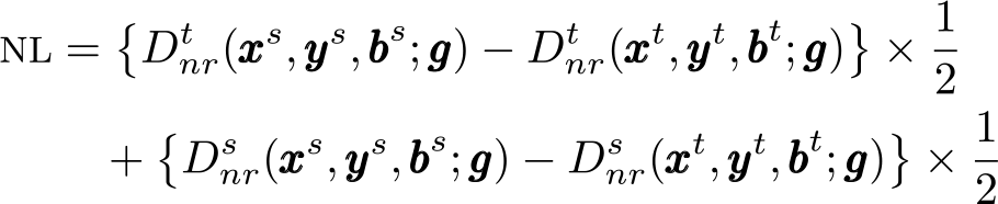
Based on the pioneering work in Chambers (2002), another productivity measure called the Luenberger productivity indicator is also widely used to account for productivity change. The Luenberger productivity indicator based on radial ddf measures is defined as

$\begin{array}{l}\text{L}=\left\{D_r^t\left({\mathit{x}}^s,{\mathit{y}}^s,{\mathit{b}}^s;\mathit{g}\right)-D_r^t\left({\mathit{x}}^t,{\mathit{y}}^t,{\mathit{b}}^t;\mathit{g}\right)\right\}\times \frac{1}{2}\\ +\left\{D_r^s\left({\mathit{x}}^s,{\mathit{y}}^s,{\mathit{b}}^s;\mathit{g}\right)-D_r^s\left({\mathit{x}}^t,{\mathit{y}}^t,{\mathit{b}}^t;\mathit{g}\right)\right\}\times \frac{1}{2}\end{array}$

Again, to avoid an arbitrary choice between base years, an arithmetic mean of a difference-based Luenberger productivity index in base year t (first difference) and s (second difference) has been taken. Productivity improvements are indicated by positive values and declines are indicated by negative values.

In the spirit of decomposition of mlpi, the Luenberger productivity indicator based on radial ddfs can also be decomposed into two component measures: an efficiency change component (Mahlberg and Sahoo 2011),

$\text{LEFFCH}=D_r^s\left({\mathit{x}}^s,{\mathit{y}}^s,{\mathit{b}}^s;\mathit{g}\right)-D_r^t\left({\mathit{x}}^t,{\mathit{y}}^t,{\mathit{b}}^t;\mathit{g}\right)$

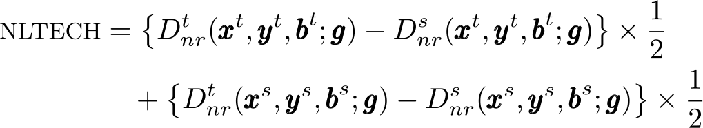
and a technical change component,

$\begin{array}{l}\text{ LTECH }=\left\{D_r^t\left({\mathit{x}}^t,{\mathit{y}}^t,{\mathit{b}}^t;\mathit{g}\right)-D_r^s\left({\mathit{x}}^t,{\mathit{y}}^t,{\mathit{b}}^t;\mathit{g}\right)\right\}\times \frac{1}{2}\\ +\left\{D_r^t\left({\mathit{x}}^s,{\mathit{y}}^s,{\mathit{b}}^s;\mathit{g}\right)-D_r^s\left({\mathit{x}}^s,{\mathit{y}}^s,{\mathit{b}}^s;\mathit{g}\right)\right\}\times \frac{1}{2}\end{array}$

The Luenberger indicator based on radial ddfs is expressed as the sum of leffch and ltech. leffch captures the average gain or loss due to the difference in technical efficiency from period s to period t. ltech captures the average gain or loss due to the shift in technology from period s to period t.

Like any radial measure of efficiency estimated using dea technologies, the ddf measure overestimates the efficiency of a firm when there are nonzero slacks that remain in the constraints after the full radial efficiency is achieved. To account for these slacks, Färe and Grosskopf (2010) proposed a slacks-based measure of efficiency based on the nonradial ddf. Another type of Luenberger indicator, called the nonproportional Luenberger indicator, can be constructed based on the nonradial ddfs (Mahlberg and Sahoo 2011).

The Luenberger productivity indicator based on nonradial ddfs is defined as

$\begin{array}{l}\text{NL}=\left\{D_{nr}^t\left({\mathit{x}}^s,{\mathit{y}}^s,{\mathit{b}}^s;\mathit{g}\right)-D_{nr}^t\left({\mathit{x}}^t,{\mathit{y}}^t,{\mathit{b}}^t;\mathit{g}\right)\right\}\times \frac{1}{2}\\ +\left\{D_{nr}^s\left({\mathit{x}}^s,{\mathit{y}}^s,{\mathit{b}}^s;\mathit{g}\right)-D_{nr}^s\left({\mathit{x}}^t,{\mathit{y}}^t,{\mathit{b}}^t;\mathit{g}\right)\right\}\times \frac{1}{2}\end{array}$

The nonproportional Luenberger productivity indicator can also be decomposed into two parts (Mahlberg and Sahoo 2011): an efficiency change component,

$\text{NLEFFCH}=D_{nr}^s\left({\mathit{x}}^s,{\mathit{y}}^s,{\mathit{b}}^s;\mathit{g}\right)-D_{nr}^t\left({\mathit{x}}^t,{\mathit{y}}^t,{\mathit{b}}^t;\mathit{g}\right)$

and a technical change component,

$\begin{array}{l}\text{NLTECH}=\left\{D_{nr}^t\left({\mathit{x}}^t,{\mathit{y}}^t,{\mathit{b}}^t;\mathit{g}\right)-D_{nr}^s\left({\mathit{x}}^t,{\mathit{y}}^t,{\mathit{b}}^t;\mathit{g}\right)\right\}\times \frac{1}{2}\\ +\left\{D_{nr}^t\left({\mathit{x}}^s,{\mathit{y}}^s,{\mathit{b}}^s;\mathit{g}\right)-D_{nr}^s\left({\mathit{x}}^s,{\mathit{y}}^s,{\mathit{b}}^s;\mathit{g}\right)\right\}\times \frac{1}{2}\end{array}$

2.4 Statistical inference for technical efficiency and productivity index

Efficiency and productivity analysis are widely applied in benchmarking (relative performance evaluations). The models introduced above are based on the dea methods, which are typically considered to be deterministic. Specifically, the efficiency or productivity is measured relative to the estimated production frontiers constructed by sample observations. Consequently, the measures of efficiency or productivity might be sensitive to the sampling variations. In view of this, researchers have devoted themselves to exploring the statistical properties of the dea-type estimators. For instance, Banker (1993) and Kneip, Park, and Simar (1998) established consistency and convergence rates of dea efficiency estimators. Kneip, Simar, and Wilson (2008) derived the asymptotic distribution of the Farrell measure of technical efficiency (one of the radial dea estimators) in cases with multiple inputs and outputs. Generally speaking, many dea-type efficiency estimators have been proposed, but few have been known for their asymptotic distribution.

To implement statistical inference for dea-type efficiency estimators, Simar and Wilson (1998) proposed a smoothed bootstrapping procedure. However, the consistency of the smooth bootstrapping method has not been proven. Based on the asymptotic theorems developed in Kneip, Simar, and Wilson (2008), Simar and Wilson presented another two consistent bootstrapping procedures for the Farrell measure of technical efficiency: the subsampling approach and the double-smooth bootstrap. Simar, Vanhems, and Wilson (2012) showed that the ddf estimators shared the known properties of the traditional radial dea estimators, and they adapted the subsampling approach and the double-smooth bootstrap to this context. In the context of nonradial dea estimators, Badunenko and Mozharovskyi (2020) proposed a bootstrap method for Russell measures of technical efficiency. Badunenko and Mozharovskyi (2016) incorporated the bootstrap procedures in their commands teradialbc and tenonradialbc.

It is worth pointing out that the bootstrap methods mentioned above mainly focus on cross-sectional data. In panel-data cases, there are some difficulties in applying the smooth and double-smooth bootstrapping methods. Because they consider the possibility of temporal correlation, they require nonparametric estimation of a high-dimensional density, which might suffer from the curse of dimensionality. On the contrary, the subsampling approach can be easily adapted to accommodate the panel-data structure by subsampling with clusters. Thus, we incorporate the subsampling approach in our command (teddf) for statistical inference.

Regarding the statistical inference for dea-based productivity indexes, Simar and Wilson (2019) established the asymptotic theorems for nonparametric Malmquist indices. Simar and Wilson (1999) proposed a bootstrap estimation procedure for obtaining confidence intervals for Malmquist indices of productivity and their decompositions. Currently, the statistical properties of the mlpi and the Luenberger productivity indicator are still unknown. Intuitively, the subsampling approach can be adapted to these contexts with the knowledge of convergence rates. Nevertheless, it is still an open issue.

3 The teddf command

teddf estimates the ddf with undesirable outputs for technical efficiency measurement.

3.1 Syntax

teddf inputvars = desirable_outputvars: undesirable_outputvars [ if ] [ in ],

dmu (varname) [time(varname) gx(varlist) gy(varlist) gb(varlist) nonradial

wmat( name ) vrs rf( varname ) window( # ) biennial sequential global

brep(#) alpha(real) tol(real) maxiter(#) saving(filename [, replace ])

frame(framename) nodots noprint nocheck ]

3.2 Options

dmu (varname) specifies the names of the dmus. dmu() is required.

time (varname) specifies the time variable for panel data.

gx (varlist) specifies the direction components for input adjustment. The order of variables specified in varlist should be the same as in inputvars. The ith variable in gx() should be the same direction as the ith variable in inputvars. By default, gx() takes the opposite of inputvars (negative one times inputvars).

gy(varlist) specifies the direction components for desirable output adjustment. The order of variables specified in varlist should be the same as in desirable_outputvars. The ith variable in gy() should be the same direction as the ith variable in desirable_outputvars. By default, gy() takes desirable_outputvars (with no alteration).

gb(varlist) specifies the direction components for undesirable output adjustment. The order of variables specified in varlist should be the same as in undesirable_outputvars. The ith variable in gb() should be the same direction as the ith variable in undesirable_outputvars. By default, gb() takes the opposite of undesirable_outputvars (negative one times undesirable_outputvars).

nonradial specifies to use the nonradial directional distance measure.

wmat(name) specifies a weight row vector for adjustment of input and output variables in the nonradial ddf. The default is wmatrix() = (1,…, 1).

vrs specifies production technology with vrs. By default, production technology with crs is assumed.

rf(varname) specifies the indicator variable that defines which data points of outputs and inputs form the technology reference set.

window(#) specifies to use window production technology with the #-period bandwidth.

biennial specifies to use biennial production technology.

sequential specifies to use sequential production technology.

global specifies to use global production technology.

brep(#) specifies the number of bootstrap replications. The default is brep(0) specifying to perform the estimator without a bootstrap. Typically, it requires 1,000 or more replications for bootstrap dea methods.

alpha(real) sets the size of the subsample bootstrap. The default is alpha(0.7) indicating to subsample N ^{0 . 7} observations out of the N original reference observations.

tol(real) specifies the convergence-criterion tolerance for LinearProgram(). It must be an integer greater than 0. The default is tol(1e-8).

maxiter(#) specifies the maximum number of iterations for LinearProgram(). It must be an integer greater than 0. The default is maxiter(16000).

saving(filename[ , replace]) specifies a filename in which to store the results.

frame(framename) specifies a framename in which to store the results.

nodots suppresses the iteration dots.

noprint suppresses display of the results.

nocheck suppresses checking for a new version. You can use this option to save time when an Internet connection is unavailable.

3.3 Dependency of teddf

teddf depends on the Mata function mm_sample(), which you can install by typing ssc install moremata (Jann 2005). Two commands, _get_version and _compile_mata, modified from Correia’s (2016) ftools package, are included to compile lgtfpch.mlib for different Stata versions.

4 The gtfpch command

gtfpch measures the tfp change with undesirable outputs by using the mlpi or the Luenberger indicator.

4.1 Syntax

gtfpch inputvars = desirable_outputvars: undesirable_outputvars [ if ] [ in ][, dmu(varname) luenberger ort(string) gx(varlist) gy(varlist) gb(varlist)nonradial wmat(name) window(#) biennial sequential global fgnz rd tol(real) maxiter(#) saving(filename [, replace ]) frame(framename)noprint nocheck ]

4.2 Options

dmu(varname) specifies the names of the dmus.

luenberger specifies to estimate the Luenberger productivity indicator. The default is the mlpi based on the radial ddf.

ort(string) specifies the orientation. The default is ort(output), which means the output-oriented productivity index. ort(input) means the input-oriented productivity index, and ort(hybrid) means the hybrid-direction productivity index.

gx(varlist) specifies the direction components for input adjustment. The order of variables specified in varlist should be the same as in inputvars. The ith variable in gx() should be the same direction as the ith variable in inputvars.

gy(varlist) specifies the direction components for desirable output adjustment. The order of variables specified in varlist should be the same as in desirable_outputvars. The ith variable in gy() should be the same direction as the ith variable in desirable_outputvars.

gb(varlist) specifies the direction components for undesirable output adjustment. The order of variables specified in varlist should be the same as in undesirable_outputvars. The ith variable in gb() should be the same direction as the ith variable in undesirable_outputvars.

nonradial specifies to use the nonradial directional distance measure.

wmat(name) specifies a weight row vector for adjustment of input and output variables in the nonradial ddf. Can be used only when nonradial is also specified.

window(#) specifies to use window production technology with the #-period bandwidth.

biennial specifies to use biennial production technology.

sequential specifies to use sequential production technology.

global specifies to use global production technology.

fgnz specifies to decompose the tfp change following the Färe et al. (1994) method.

rd specifies to decompose the tfp change following the Ray and Desli (1997) method.

tol(real) specifies the convergence-criterion tolerance for LinearProgram(). It must be greater than 0. The default is tol(1e-8).

maxiter(#) specifies the maximum number of iterations for LinearProgram(). It must be greater than 0. The default is maxiter(16000).

saving(filename [, replace ]) specifies a filename in which to store the results.

frame(framename) specifies a framename in which to store the results.

noprint suppresses display of the results.

nocheck suppresses checking for a new version. You can use this option to save time when an Internet connection is unavailable.

5 Example

To exemplify the use of the commands described above, we use an input–output dataset of China’s provinces for the period of 2013–2015 (Yan et al. 2020). The dataset includes three input variables (capital, labor, and energy), one desirable output (real gross domestic product), and one undesirable output CO₂ emissions). The data are as follows.

5.1 Application of teddf

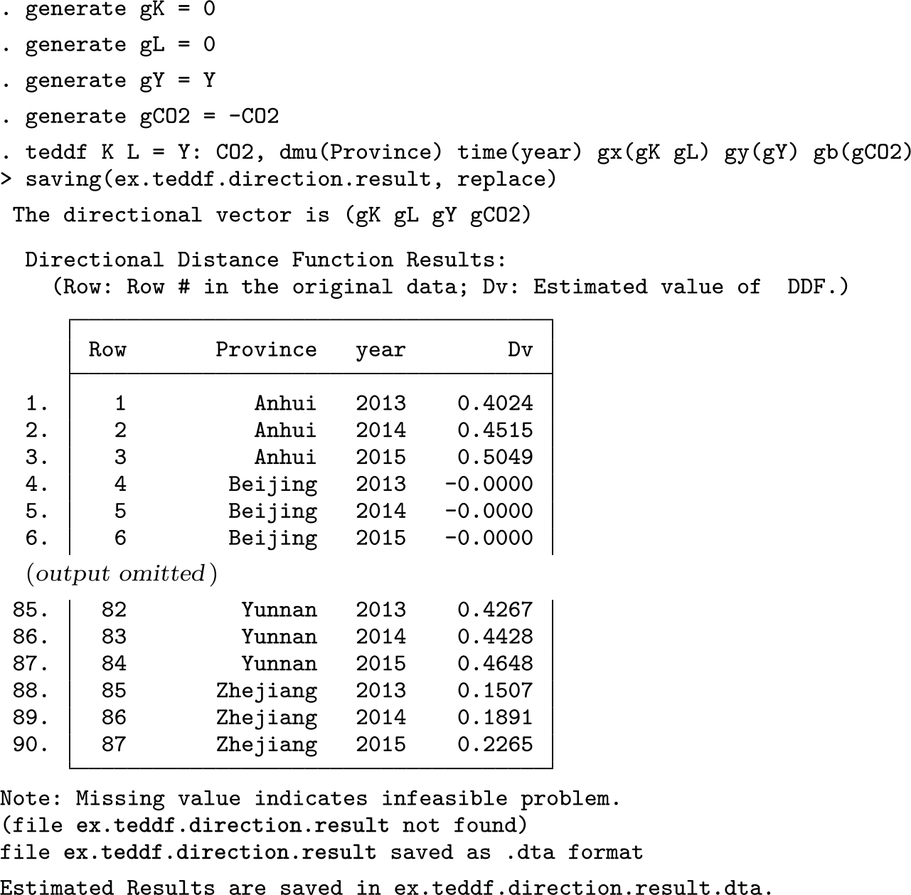
The estimation of the ddf model proposed by Chung, Färe, and Grosskopf (1997) is as follows. The corresponding results are displayed below the executed command. The Dv variable stores the values of the ddf of the dmus. Note that save(ex.teddf.result) saves the results in a new data file named ex.teddf.result.dta.

We can customize the directional vector as follows:

What follows is an application of teddf to fit the nonradial ddf model. The Dv variable stores the values of the nonradial ddf of the dmus. The B_K, B_L, B_CO2, and B_Y variables store the reduction proportion of the inputs (K, L) and undesirable outputs (CO2), and the expansion proportion of the desirable output (Y), respectively.

We can customize the weight matrix as follows:

5.2 Application of gtfpch

We first apply gtfpch to estimate the mlpi to measure the green tfp growth of China’s provinces. Regarding the results, TFPCH stores the values of the mlpi; TECH and TECCH are the two decomposition terms of mlpi, describing technical efficiency change and technological change, respectively. We implement the estimation based on the global technology benchmark by specifying the global option.

Alternatively, gtfpch can be used to estimate the Luenberger productivity indicator.

6 Conclusion

With the increasing demand for improving sustainability at the macro and micro levels, scholars and managers recognize that it is becoming more important to consider undesirable output in efficiency and productivity analysis. However, Stata, as one of the leading packages for economic analysis, has not provided comprehensive tools to measure technical efficiency and tfp change when considering undesirable outputs. As an attempt to fill this gap, we introduced two new commands that perform estimations for nonparametric frontier models with undesirable outputs.

teddf estimates the ddf with undesirable outputs for technical efficiency measurement. Both radial Debreu–Farrell and nonradial Russell measures can be calculated under different assumptions about the production technology, for example, window, biennial, sequential, or global production technology. gtfpch measures the tfp change with undesirable outputs by using the mlpi or the Luenberger indicator. Two specifications to decompose the tfp change were given. Some empirical examples were presented to show the usage of the two commands.

Finally, note that the models we introduced are dea-type estimators, which might be sensitive to sampling variation. Thus, the statistical inference in this context is critical. However, there are still many open issues in both theory and application.

8. Programs and supplemental materials

Supplemental Material, sj-zip-1-stj-10.1177_1536867X221083886 - Measuring technical efficiency and total factor productivity change with undesirable outputs in Stata

Supplemental Material, sj-zip-1-stj-10.1177_1536867X221083886 for Measuring technical efficiency and total factor productivity change with undesirable outputs in Stata by Daoping Wang, Kerui Du and Ning Zhang in The Stata Journal