Interpreting logit models

Abstract

The parameters of logit models are typically difficult to interpret, and the applied literature is replete with interpretive and computational mistakes. In this article, I review a menu of options to interpret the results of logistic regressions correctly and effectively using Stata. I consider marginal effects, partial effects, (contrasts of) predictive margins, elasticities, and odds and risk ratios. I also show that interaction terms are typically easier to interpret in practice than implied by the recent literature on this topic.

1 Introduction

Applied researchers estimate logit models to infer the causal effect of one or more treatments (for instance, infertility) on the probability of a binary outcome (joining the labor force) for a population of interest (married women). In contrast to the linear probability model (LPM), the logit model always produces predicted probabilities within the meaningful range [0, 1]. “From a practical perspective,” however, “the most difficult aspect of logit […] models is presenting and interpreting the results” (Wooldridge 2020, chap. 17). Researchers often mislabel their findings or fail to present them in an intuitive and compelling fashion. Computational mistakes are not uncommon. This pedagogical review article summarizes and illustrates a menu of options to interpret the coefficients of logit models correctly and effectively. ¹ It covers approaches—for instance, elasticities and risk ratios—that are rarely discussed systematically in econometrics textbooks. In addition, it shows that interaction terms in logit models are much easier to interpret in practice than implied by the recent literature on this topic (Ai and Norton 2003; Norton, Wang, and Ai 2004). Readers may refer to the more primary sources cited here for additional details.

Conditional on a vector X of covariates, the expected value of a binary dependent variable (Y ) equals the probability of a positive outcome: E(Y_i |X _i ) = 1 × P (Y_i = 1|X _i ) + 0 × [1 − P (Y_i = 1|X _i )] = P (Y_i = 1|X _i ). In the LPM, this conditional probability is given a linear specification,

$P\left(Y_i=1\mid X_i\right)=X_i\beta$

and the coefficients (β) are estimated by ordinary least squares. In reality, however, probabilities cannot exceed the [0, 1] interval by definition, and the data-generating process is nonlinear. Thus, a commonly used functional form is the logistic function, which is sigmoid shaped and has limit 0 and 1 as X _iβ tends to −∞ and +∞, respectively:

$P\left(Y_i=1\mid X_i\right)=\frac{1}{1+e^{-X_i\beta }}$

1

In Stata, the maximum likelihood estimates of the β’s in (1) can be obtained with the logit command. ²

To illustrate, I estimate a labor supply model using survey data on 753 married women (Mroz 1987). inlf (“in labor force”), the outcome, is an indicator variable that takes the value 1 if a woman reports working for a wage and 0 otherwise. nokid takes the value 1 if a woman has no children younger than six years old at the time of the survey and 0 otherwise. ³ nwifeinc (“nonwife income”) measures the husband’s annual earnings, in thousands of euros.

2 Marginal effects (continuous covariates)

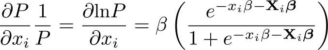
The impact on P (Y_i = 1|x_i, X _i ) of a “marginal” (infinitesimally small) change in x_i , a continuous variable, can be obtained by differentiating (1) with respect to x_i ,

$\frac{\partial P}{\partial x_i}=\beta \left[\frac{e^{-x_i\beta -X_i\beta }}{{\left(1+e^{-x_i\beta -X_i\beta }\right)}^2}\right]$

2

where β denotes the coefficient on x_i . This quantity measures the “marginal effects” of x_i (see also Williams [2012] for an introductory account). First, note that in contrast to the linear probability model, where ∂P/∂x_i = β, the value of ∂P/∂x_i given by (2) is not equal to β, because it also depends on the scale factor in brackets. Thus, the coefficients reported in the logit output are not marginal effects and do not have a probability interpretation. Second, note that the scale factor is a function of x_i , the variable of interest, and the other covariates. Thus, ∂P/∂x_i is not constant as in the LPM but varies for different values of x_i and X _i . To obtain a summary statistic, we could evaluate ∂P/∂x_i at the mean values of x_i and X _i . This is called marginal effects at the means. Until recently, this was the most common approach in applications: ⁴

. quietly margins, dydx(nwifeinc) at means

Yet, when some of the covariates (nokid) are binary, the sample means do not describe any particular woman in the sample. Thus, it makes better sense to “average over” the covariates—that is, compute ∂P/∂x_i at the values of x_i and X _i actually observed in each woman in the sample (asobserved in Stata jargon) and then take an average across observations. The quantity thus obtained measures the average marginal effects. This is now Stata’s default option:

On average, a 1,000-euro increase in a married man’s annual income leads to a 0.49 percentage-point drop in the probability that his wife might join the labor force.

3 Predicted probabilities (continuous covariates)

Very often, a more informative way to convey the results is to plot $\widehat{P}(Y_i= 1|X_i)$ , the predicted probability of being in the labor force, conditional on selected values of covariates. Here we allow nwifeinc to range between 0 and 100,000 euros (the sample range), distinguishing between women with and without children. Users could graph $\widehat{P}$ using a combination of margins and marginsplot (see StataCorp [2021, 1501–1504] for details). Yet a more flexible, user-friendly approach is provided by Royston’s (2013) mcp (or marginscontplot) command, which may be downloaded from the Stata Journal website (type net search marginscontplot and select gr0056). This command plots the response variable (here the probability that inlf = 1) at given values of the predictors, averaging over the remaining covariates, if there are any. The fixed values of the predictors can be specified with the at1( numlist ) and at2( numlist ) options, which in this example refer to nwifeinc and nokid, respectively:

Figure 1.

Predicted probabilities of being in the labor force (inlf = 1) with 95% confidence interval Figure 1 ⁵ allows us to read off the vertical axes the probability of labor-force participation at given values of nokid and nwifeinc and to clearly visualize the negative effect of nwifeinc (the downward slope of the curves).

As an alternative (or in addition) to plotting a diagram, users can also obtain a table of predicted probabilities. This can be accomplished with margins—or, more conveniently, with Long and Freese’s (2014) mtable command, which is part of the spost13 suite of commands downloadable from J. Scott Long’s Indiana University webpage (type net search spost13 and select spost13_ado). This command uses margins behind the scenes to construct tables of predictions. As always, users can specify at( atspec ) options to indicate which predicted probabilities should be displayed and in what order. For instance, some of the probabilities shown on the vertical axis of figure 1 may be obtained by typing

For instance, the probability that a childless (nokid = 1) woman with a low-income husband (nwifeinc = 20) is economically active is 62%.

4 Logit versus LPM

Note that, consistent with (2), the slope of the curves shown in figure 1—the marginal effects of nwifeinc—is a function of nwifeinc. Yet, in this application, it is clear that the marginal effects are fairly constant across most of the distribution of earnings, implying a near-linear relationship between P and nwifeinc. ⁶ Thus, in this particular case, a simple LPM specification might provide a satisfactory approximation of the true relationship:

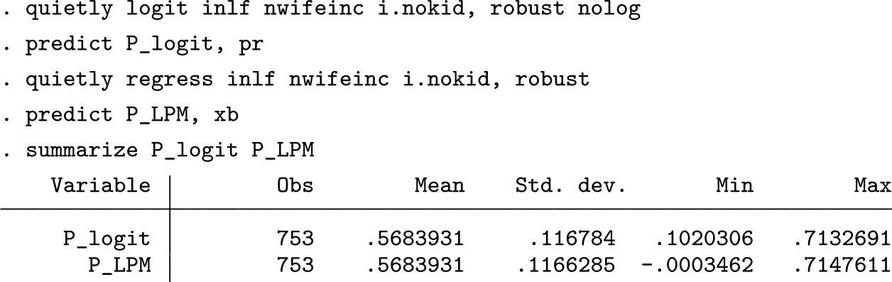
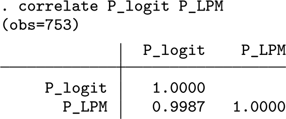
The estimated coefficient on nwifeinc (−0.00479) is fairly close to the average marginal effects implied by the logit model (−0.00489). The predicted probabilities are also very similar across the two models, although only the logit probabilities are strictly within the meaningful 0–1 range:

Of course, when the data-generating process is highly nonlinear, the discrepancy between LPM and logit may be much greater, and the predicted probabilities obtained from LPM highly misleading, if meaningful at all (see also Allison [2017]).

5 Partial effects (continuous covariates)

In nonlinear models, marginal effects provide a good approximation of the impact of a change in x_i only if the change is “small”. Suppose we would like to know how much less likely a woman is to join the labor force if her husband’s annual income goes up by one standard deviation (δ = 11635 euros). In applications, a very common approach is to multiply 0.49 by 11.63 and conclude that P declines by 5.70 percentage points. Yet, since 11,635 is far from a “marginal” increment, this computation is technically incorrect. For a discrete change in x_i , researchers should estimate the (average) difference in predicted probabilities: ⁷

$P\left(Y_i=1\mid x_i+\delta ,X_i\right)-P\left(Y_i=1\mid x_i,X_i\right)=\frac{1}{1+e^{-\left[\left(x_i+\delta \right)\beta +X_i\beta \right]}}-\frac{1}{1+e^{-\left(x_i\beta +X_i\beta \right)}}$

This calculation cannot be easily accomplished using margins. Instead, researchers can use the mchange command developed by Long and Freese (2014). ⁸ Exploiting the margins command behind the scenes, mchange returns the effects of marginal or discrete changes in a specified treatment variable (here nwifeinc), while providing a user-friendly interface. For marginal effects, users can request the amount(marginal) option. For the partial effect of a standard-deviation change (= δ) in the specified regressor, the amount(sd) option should be invoked:

For other discrete changes, users can customize the magnitude of δ by specifying the delta( # ) option, which overrides amount(sd).

In this example, the correctly estimated partial effect (5.76) is close to the figure obtained by multiplying the average marginal effects by the standard deviation (5.70). Yet, when the estimated conditional probability is highly nonlinear in the covariates, this back-of-the-envelope calculation may produce seriously misleading estimates. Users are therefore advised to always compute the correct partial effects as the default option.

6 Margins and contrasts of margins (binary covariates)

When the treatment x_i is binary (for example, nokid), or more generally a factor variable, researchers can evaluate the magnitude of the estimated effect in at least two ways. First, they may compute the predicted probability of a positive outcome (“predictive” or “conditional margins” in Stata jargon), treating all the women in the sample as if they had $\left[\widehat{P}[(Y_i=1|x_i=1,X_i)]\right]$ or had no kids $\left[\widehat{P}[(Y_i=1|x_i=0,X_i)]\right]$ . Second, researchers can calculate the difference between these two predicted probabilities, which is known in Stata jargon as the “contrast of margins”. ⁹ Again, users can either average over the covariates (X _i ), as we do here, or alternatively hold them fixed at specific values by requesting the at( atspec ) or atmeans option:

While the i. prefix requests an indicator for each level (category) of the variable nokid, the r. prefix requests a contrast between each level (in this case, just nokid = 1) and the reference category (nokid = 0). On average, 62 out of 100 women without kids join the labor force, while only 36 women with kids do so (predictive margins). Accordingly, childlessness increases a women’s likelihood of joining the labor force by almost 26 percentage points (contrast of margins). This contrast is significantly different from zero.

Note that the contrast of margins is typically defined as the marginal effects of the factor variable. Thus, an identical estimate may be obtained by typing margins, dydx(nokid). Here the Stata output helpfully reminds users that dy/dx for factor levels is the discrete change from the base level, rather than the instantaneous (marginal) rate of change. ¹⁰ A very common mistake, which is also to be found in the Stata manual (for instance, see StataCorp [2021, 1468]), is to conclude based on the estimated contrast of margins that childless women are almost 26% more likely to join the labor force. This is wrong because it implies an elasticity rather than a marginal effect.

7 Elasticities (continuous and binary covariates)

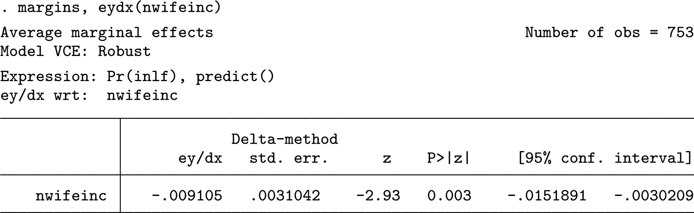
In some cases, it may be more appropriate or informative to report the relative (that is, percentage) change in probability, rather than the absolute change, induced by a treatment. If x_i is continuous (for example, nwifeinc), the percentage change is given by the (semi)elasticity:

$\frac{\partial P}{\partial x_i}\frac{1}{P}=\frac{\partial \ln P}{\partial x_i}=\beta \left(\frac{e^{-x_i\beta -X_i\beta }}{1+e^{-x_i\beta -X_i\beta }}\right)$

On average, a 1,000-euro increase in the husband’s income leads to a 0.91% decrease in the probability that the wife might join the labor force.

When the treatment variable (for example, nokid) is binary, the strict definition of relative change leads to the following expression for the response:

$\frac{P\left(Y_i\mid x_i=1,X_i\right)-P\left(Y_i\mid x_i=0,X_i\right)}{P\left(Y_i\mid x_i=0,X_i\right)}=\frac{1+e^{-X_i\beta }}{1+e^{-\beta -X_i\beta }}-1$

3

For a small ΔP, log differences approximate percentage changes. Thus, an alternative formula for the response is

$\ln P\left(Y_i\mid x_i=1,X_i\right)-\ln P\left(Y_i\mid x_i=0,X_i\right)=\ln \left(1+e^{-X_i\beta }\right)-\ln \left(1+e^{-\beta -X_i\beta }\right)$

4

Perhaps unfortunately, Stata uses (4), not (3), to run margins, eydx(i.nokid) after logit. ¹¹ There is no shorthand command to compute (3), and users wishing to estimate the “exact” definition of relative change should code this expression manually using margins‘s expression( pnl_exp ) option (see also Uberti [2017]). I illustrate this procedure more explicitly in sections 8 and 9 below.

Estimates based on these definitions of “relative change” are presented in table 1. Based on (3), childless women are 72% more likely to join the labor force. For each woman, the change in probability is measured relative to the base level—that is, the probability of a positive outcome for that woman assuming that she had kids (x_i = 0). Then, the percentage changes for all the different women in the sample are averaged. Based on (4), childless women are 54% more likely to participate in the labor force. In this case, ΔP (= 0.256) is not exactly “small”, and so (4) does not provide a good approximation of percentage change.

Table 1.

Alternative measures of “relative change”

Response formula	Estimate	(s.e.)
(3) N− 1Σ{ΔP/P (Yi |xi = 0, X i )}	0.721	(0.199)
(4) N− 1Σ(ΔlnP )	0.541	(0.115)
(3a) $N^{-}{ }^1\Sigma (\Delta P)/\overline{P}(Y_i|x_i,X_i)$	0.450	(0.078)
(3b) N− 1Σ{ΔP/P (Yi |xi, X i )}	0.477	(0.093)

NOTES: ΔP = P (Y_i|x_i = 1, X _i ) − P (Y_i|x_i = 0, X _i ). N refers to the number of observations, and the summation operator is over all observations i.

There are more ways to define the notion of relative change. Researchers, for instance, could measure the average change in probability (that is, the contrast of margins) relative to the average observed probability $\overline{P}$ of a positive outcome (the mean of the dependent variable). This approach, denoted as (3a) in table 1, is common in applications because it is easy to compute. Lastly, researchers may compare the change in probability for each woman with the expected probability of a positive outcome for that woman (who may or may not have kids) and then take an average (3b).

The estimates of (3a) and (3b) are quite similar to each other, and to the log difference (4). Yet they are all considerably smaller in magnitude than the estimate of average percentage change strictly defined—that is, (3). Researchers should decide case by case which number is most meaningful, if any.

8 Odds and risk ratios (binary covariates)

So far, the effects of binary treatments were presented on an additive scale. Sometimes, it may be more informative to present the results on a multiplicative scale (Buis 2010). For the logit model, the most common options are odds and risk ratios. The odds are defined as the ratio of the probability of an event occurring to the probability of it not occurring: P (Y_i = 1|x_i, X _i )/P(Y_i = 0|x_i, X _i ), where x_i is a binary variable. Thus, the odds of a woman joining the labor force are the expected number of women in the labor force for every woman that is not in the labor force. It follows that, for a change in x_i from 0 to 1, the odds ratio is given by

$\text{ Odds ratio }=\frac{P\left(Y_i=1\mid x_i=1,X_i\right)/P\left(Y_i=0\mid x_i=1,X_i\right)}{P\left(Y_i=1\mid x_i=0,X_i\right)/P\left(Y_i=0\mid x_i=0,X_i\right)}=e^{\beta }$

5

where β is the coefficient on x_i . This expression is attractive because it may be computed by simply exponentiating β. ¹² To see this, simply substitute (1) into (5), and simplify the fractions. Note that, from (5), it also follows that the point estimates returned by logit (the β’s) are the odds ratios in logs, or log odds, which do not admit of a straightforward interpretation.

For nokid, the odds ratio can be obtained in postestimation simply by typing

The odds of being in the labor force—the number of women in the labor market for every woman in home production—are almost three times higher for childless women than for women with children. Alternatively, users could call the logit command with the or option (or type logistic instead of logit). These commands return all the estimated coefficients in exponentiated form. The problem, of course, is that some of the variables may be continuous, and exponentiating the coefficient of a continuous variable is not very useful for interpretation.

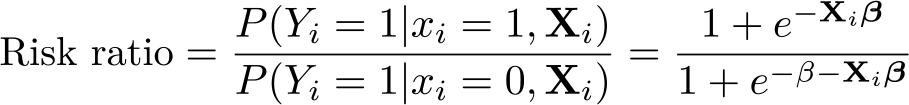
Often, reporting the ratio of two probabilities—the risk ratio—may be preferable to reporting the ratio of two odds:

$\text{ Risk ratio }=\frac{P\left(Y_i=1\mid x_i=1,X_i\right)}{P\left(Y_i=1\mid x_i=0,X_i\right)}=\frac{1+e^{-X_i\beta }}{1+e^{-\beta -X_i\beta }}$

Note that this quantity equals one plus the relative change given by (3). Just like relative changes, risk ratios are laborious to calculate in Stata:

On the upside, they often provide a clear and compelling formulation of the results: childless women are 1.72 times (72%) more likely to be in the labor force than women with children. When the predicted probabilities are small (which is not the case in our example), odds ratios approximate risk ratios (Buis 2010). In general, however, they are different quantities and should not be confused.

9 Interaction terms

Binary choice models may also include interaction (or higher-order) terms. For instance, the effect of the husband’s income on a woman’s labor-supply decision may be thought to depend on the woman’s level of education. While women with few years of education (educ) may leave the labor market when the husband begins to earn well, highly educated women with career ambitions may be more likely to stay on irrespective of their husband’s income. This argument motivates the inclusion of a multiplicative interaction term between the treatment of interest (nwifeinc) and the effect modifier (educ), leading to

$P\left(Y_i=1\mid X_i\right)=L\left(u_i\right)=L({\beta }_{1}nwifeinc{ }_i+{\beta }_{2}educ{ }_i+{\beta }_{12}nwifeinc{ }_i\times educ{ }_i+\gamma nokid{ }_i)$

6

where L denotes the logistic function (= 1/1 + e^{− u} ) and u is a linear index of the covariates:

A Wald-type test suggests that nwifeinc and nwifeinc × educ are jointly significant. Relying on intuitions carried over from linear models, we may find it tempting to look at the positive sign on the estimated coefficient on nwifeinc × educ and conclude that an additional year of education lessens the negative impact of the husband’s earnings on the wife’s labor-supply decision, in line with expectations. Yet it is now well known that, in nonlinear models, this conclusion is flawed (Ai and Norton 2003).

The reason is simple, though far from self-evident. By definition, the interaction effect describes how much a marginal change in educ modifies the impact of the treatment, here nwifeinc: ∂{∂P/∂(nwifeinc)}/∂(educ) = ∂ ² P/∂(nwifeinc)∂(educ). ¹³ In the LPM, this cross-partial derivative is constant and equal to ∂P/∂(nwifeinc× educ), the coefficient on the multiplicative term. In nonlinear models such as logit, however, this equality does not hold in general. Furthermore, similar to the other expressions discussed so far, ∂ ² P/∂(nwifeinc)∂(educ) also depends on the values of covariates. Indeed, even its sign need not be the same as the sign of the estimated coefficient on the multiplicative term. Ai and Norton (2003) derive formulas for ∂ ² P/∂(nwifeinc)∂(educ) for logit (and probit) models.

In Stata, the correct interaction effect (∂ ² P/∂(nwifeinc)∂(educ)) after logit can be computed with the inteff command developed by Norton, Wang, and Ai (2004) and downloadable from the Stata Journal’s website (type net search inteff and select st0063). ¹⁴ This command (which does not support factor-variable notation) produces a numerical estimate of the average interaction effect (_logit_ie in the output below), treating all the individuals asobserved:

Note this estimate is an average: as already mentioned, ∂ ² P/∂(nwifeinc)∂(educ) is different for different values of covariates. Here the mean (0.0004244) conceals a large amount of heterogeneity, with the magnitude of the interaction effect ranging between −0.00099 and 0.00106 depending on the values of covariates. Somewhat unfortunately, the statistics reported as _logit_se and _logit_z (third column) refer to the average standard error and z statistic, rather than the standard error and z statistic of the average interaction effect reported just above.

To be sure, the inteff command was developed before factor-variable notation, and margins were introduced in Stata 11 (2009). Most of inteff‘s output can now be reproduced more flexibly, albeit more laboriously, using margins (see below).

In practice, however, things are even easier. In many (probably, most) settings, the researcher is not primarily interested in how much the effect of a treatment changes in response to a marginal change in the modifier (that is, the interaction effect) but in what the treatment effect actually is for various degrees of exposure to the modifier. Thus, the derivative of (6) with respect to nwifeinc is often more useful for interpretation than ∂ ² P/∂(nwifeinc)∂(educ): ¹⁵

$\frac{\partial P}{\partial \left(nwifeinc\right)}=\left({\beta }_1+{\beta }_{12}edu{c}_i\right)L^{\prime }\left(u\right)=\left({\beta }_1+{\beta }_{12}edu{c}_i\right)\left(\frac{e^{-u_i}}{{\left(1\hspace{0.17em}+\hspace{0.17em}{e}^{-u_i}\right)}^2}\right)$

7

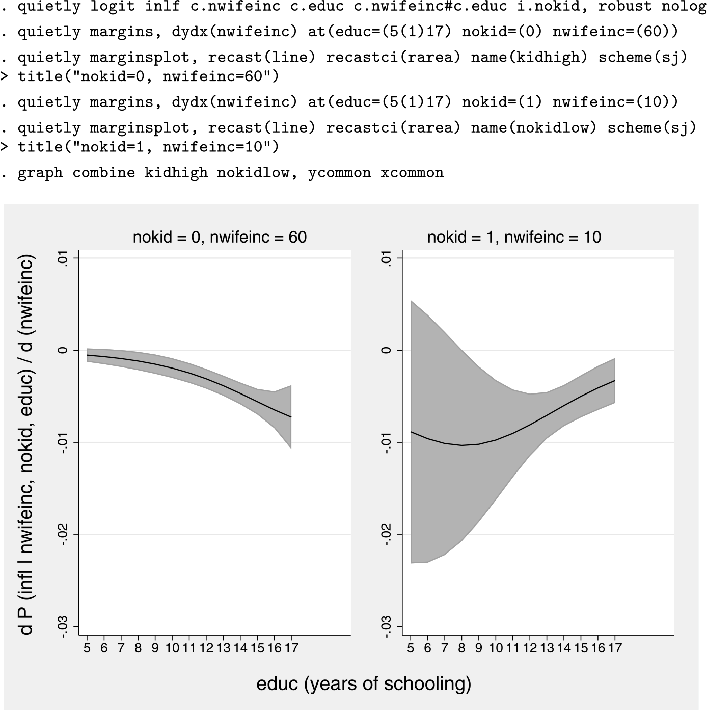
As is standard in applications involving linear models, ∂P/∂(nwifeinc) can easily be plotted as a function of educ, the effect modifier, averaging over the remaining covariates. Of course, researchers may also hold some of or all the covariates fixed at representative values, or at the means, if they wish. This is what we do here. Figure 2 ¹⁶ evaluates (7) for a) women with kids (nokid = 0) and wealthy husbands (income of 60,000 euros); and b) childless women with husbands on very low incomes (10,000 euros).

Figure 2.

Average marginal effects of nwifeinc with 95% confidence interval

It is clear from figure 2 that whether ∂P/∂(nwifeinc) is upward or downward sloping—that is, whether ∂ ² P/∂(nwifeinc)∂(educ), the interaction effect, is positive or negative—depends on the values of covariates. For childless women with husbands on low incomes (right panel, figure 2), education mitigates the substitution effect triggered by the husband’s income [∂ ² P/∂(nwifeinc)∂(educ) > 0], at least past a given point (educ ≅ 8). This finding is in line with theoretical expectations. For women with kids and wealthy husbands (left panel, figure 2), things work differently. An additional year of schooling amplifies the substitution effect of the husband’s earnings—that is, it makes the estimated effect more negative [∂ ² P/∂(nwifeinc)∂(educ) < 0]. This finding runs counter to theoretical expectations.

In many (probably, most) applications, a diagram along the lines of figure 2 will provide more than enough insights to interpret the regression results, with no need to compute the interaction effect itself using inteff. Some researchers, however, may wish to take it a step further and report the magnitude and statistical significance of ∂ ² P/∂(nwifeinc)∂(educ), the interaction effect, at the representative values of covariates displayed in figure 2. This calculation cannot be accomplished by inteff. Rather, users should differentiate (7) with respect to educ (see Ai and Norton [2003, 124]) and code the resulting formula for the response manually:

$\begin{array}{c}\frac{{\partial }^{2}P}{\partial \left(nwifeinc\right)\partial \left(educ\right)}={\beta }_{12}{L}^{\prime }(u)+\left({\beta }_1+{\beta }_{12}educ{ }_i\right)\left({\beta }_2+{\beta }_{12}nwifeinc{ }_i\right)L^{″}(u)\\ \begin{array}{l}={\beta }_{12}L(u)\left\{1-L(u)\right\}+\left({\beta }_1+{\beta }_{12}educ{ }_i\right)\left({\beta }_2+{\beta }_{12}nwifeinc{ }_i\right)\hfill \\ \hspace{0.17em}L(u)\left\{1-L(u)\right\}\left\{1-2L(u)\right\}\hfill \end{array}\end{array}$

8

For instance, for the left panel in figure 2, the interaction effect (the slope of the curve) can be obtained by first defining a macro for L(u) and then coding (8) into margin‘s expression( pnl_exp ) option:

By dropping the at(nokid=0 nwifeinc=60 educ=(5(3)17)) option from the command above, users can also replicate the average interaction effect outputted by inteff (= 0.0004244). Usefully, they can also obtain an estimate of the standard error of this average effect (= 0.0007605), which is not returned by inteff.

In sum, margins (and in particular its expression() option) expands the range of possibilities made available by inteff (only at the cost of making the coding a bit more laborious). Yet I suggest that things are much easier in practice. Describing how the marginal effects of the variable of interest (nwifeinc) vary at different values of the effect modifier (educ), as in figure 2, is quicker and usually more informative than reporting interaction effects [that is, the values returned by (8)].

10 Conclusion

When fitting binary choice models, applied researchers should carefully consider the best way to interpret the coefficients, repressing a knee-jerk temptation to compute and report marginal effects indiscriminately after running a logit or probit regression. Plotting the predicted probabilities is often a visually effective solution. When some of the regressors are binary, predictive margins (that is, the predicted probabilities) and their contrasts (difference) are the way to go. Elasticities can be a tricky option because percentage changes in probability can be difficult to grasp intuitively and are sensitive to the choice of response formula. By contrast, risk ratios can often provide an effective metric to convey the results, although they are tedious to compute in Stata. In the presence of interaction terms, things are actually easier in practice than implied in the recent literature on this topic: researchers can simply use margins to plot the marginal effects of the treatment of interest as a function of the effect modifier. Usually, the resulting diagram conveys the nature of heterogeneous effects in a clear and intuitive fashion.

Logit (and probit) provides a more accurate description of binary choice processes than the LPM (Allison 2017). With a little effort, logit can be combined with margins or other related postestimation commands, or both, to obtain interpretable numerical estimates. Of course, when (and only when) a linear approximation can be made with little loss of information, as in the example discussed in this article, researchers can fall back on the LPM and estimate by ordinary least squares, simplifying the interpretation of the coefficients. The tools reviewed in this article, however, suggest that interpreting logit models in Stata is not prohibitively hard and that logit (rather than the LPM) should be the default approach.

Supplemental Material

Supplemental Material, sj-zip-1-stj-10.1177_1536867X221083855 - Interpreting logit models

Supplemental Material, sj-zip-1-stj-10.1177_1536867X221083855 for Interpreting logit models by Luca J. Uberti in The Stata Journal