1 merge versus joinby
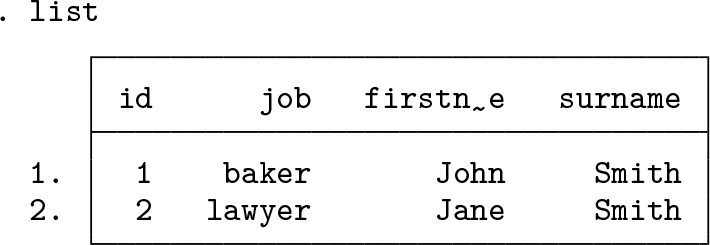
The merge command is one of Stata’s most used commands and works fine as long as the match key is unique in one of the datasets (that is, merge 1:1, 1:m, or m:1 situations). However, when the match key contains duplicates in either dataset, Stata gives an error message saying that the key variable(s) do not uniquely identify observations in master or using dataset. An example can clarify. In jobs.dta, we have two individuals. The first individual is a baker, and the second individual is a lawyer. The first and last names of each individual are included in names.dta.

Merging these two datasets is straightforward in Stata:

The merge 1:1 shows that John Smith is a baker and Jane Smith is a lawyer.
Things get tricky if we want to add information on the children of these workers. John and Jane Smith have two children together, Ken and Sue Smith.

children.dta can be linked to names.dta through their common surname, Smith. The Smith family consists of multiple parents and multiple children, suggesting we would need a merge m:m. However, this will not assign both children to both parents! Rather, merge m:m produces the nonsensical result below:

It linked the first parent to the first child and the second parent to the second child, rather than assigning both children to both parents.
Stata will not return an error message in this situation. Indeed, one motivation to write this tip was that we fear there are articles out there whose authors unwittingly ran a merge m:m. This is especially relevant in large population datasets that include millions of parents and children.
Instead, this situation requires the joinby command. Using the joinby command, we can add the information of each child to each parent.

2 Stata example
Stata provides example parent.dta and child.dta datasets to test joinby yourself.

We start by demonstrating the correct approach using joinby:

The joined dataset correctly contains information on all parents (four) and on all their children (four in total). By default, joinby excludes unmatched observations. In this case, that means parents 10 and 15 and child 5 are not present in the joined dataset. This behavior can be changed through the unmatched() option.

Just like merge, joinby also provides options to handle variables present in both datasets. By default, joinby retains the values of the primary dataset (compare x1 above). Specifying the option update will update missing values with any nonmissing values in the secondary dataset. Adding the replace option will overwrite primary values with secondary values unless the latter are missing.
Contrast this result to the merge m:m outcome, where we specify keep(match) to mimic joinby’s default of excluding unmatched observations.

The merge m:m result below is extremely dangerous. In the first family (ID 1025), it assigned the first child (ID 3) to the first parent (ID 11) and all remaining children to the second parent (ID 12). In the second family, however, it correctly assigned the single child (ID 2) to both parents (IDs 13 and 14). As a result, if you manually checked the second family’s results, you would assume merge m:m did exactly what you wanted even though it used a different allocation rule for the first family.

The examples above highlight that you should (almost) never use merge m:m when the key match variable does not uniquely identify observations in both the master and the using datasets. Instead, if you want to assign all observations of the using dataset to all observations in the master dataset (for example, all children to all their parents), then joinby does exactly that.

