Stata tip 144: Adding variable text to graphs that use a by() option

1 The problem

Graphs may be enhanced using a variety of title options, as explained in the help for title options. When the g raph command also uses a by() option naming a variable to categorize data, the subtitle() automatically shows the value on that variable (or the associated value label if defined) of the particular group of observations being shown in each panel.

You might wish to add further text that varies from panel to panel. In particular, you might wish for scope to vary text in a note() or caption() from panel to panel. At the time of writing (Stata 17), that scope is not available. Either a note or caption applies to the entire display, or (less helpfully) the same note or caption is repeated for each panel.

This tip explains two alternative methods for adding text that varies informatively. A third method, not illustrated here, is to produce individual graphs as desired and then use graph combine. The advice here is a sequel or complement to an earlier tip (Cox 2011), which pointed out that title and legend options can be moved away from their default positions and placed within the plot region.

Our first example concerns how to add information on the number of observations to a scatterplot (figure 1).

Figure 1.1.

This is a simple example of a scatterplot using by(). How do we add extra text in each panel, say, flagging the number of observations in each group?

In all this, there is a permanent tension between making a graph more informative and wanting to avoid crowding and clutter. Much good advice (for example, Cleveland [1994]; Wilke [2019]) is on its face contradictory. It is a good idea to employ direct labeling, showing text right by data points or lines, rather at some distance as part of a key or legend. It is also a good idea to show the data clearly without congestion from extra text, so that the plot region is easy to scan and scrutinize. Circumstances and tastes affect choices, and the methods here are part of the flexibility you have as a graph designer.

2 Solution 1: Use an extra variable containing text as a marker label

We could create an extra string variable containing the text we need and then show that as a marker label. The marker label does not have to be associated with any variable already shown on the plot. On the contrary, it is often better to place the text well away from data points or lines in the plot region.

Looking at the graph in figure 1 suggests that a good location would be at mpg = 11, weight = 1800. (In practice, you may need some experimentation to find a position that seems good.) In our example, there are no missing values associated with mpg or weight, so we can get the number of observations shown from the number of observations N, which under by: is determined groupwise. (See, for example, Cox [2002] on by: if all this is new to you.).

Had there been any missing values, a more general technique would be to count the number of observations with nonmissing values:

The reasoning here: !missing(mpg, weight) returns 1 if both mpg and weight are not missing—the condition that defines an observation to be shown on the scatterplot—and 0 otherwise. Hence, adding results from that function across groups of observations puts the counts in a new variable.

An important flag: The Stata Markup and Control Language annotation instructing graph to show n in italic points up facilities for markup, including not just italic and bold fonts but also often-needed elements such as mathematical and other symbols, Greek characters, and subscripts and superscripts. See the help on SMCL and on text for the details.

We can now draw our graph. We are superimposing a plot of y versus x—which does just one thing, show extra text—on the original plot of mpg versus weight. A detail to fix is that with two y variables and two x variables, graph does not know what we want as axis titles. So here we reach in and insist on showing the variable labels for mpg and weight. Had no variable labels been defined, we could have used the variable names. In either case, we could have specified any other text that appeals for the axis titles. Similarly, we suppress the legend that would otherwise spring into existence: two y variables are being shown, but we do not need a legend entry for either. Figure 2 is the result.

Figure 2.1

A string variable shown as marker labels is here used to add text in each panel indicating the number of observations shown. The value of the string variable is constant in each group, and variable from group to group, so the text shown matches that.

3 Solution 2: Modify the values or value labels of the by() variable

A second solution is to add information that will appear in the subtitles. Let’s go through the possibilities:

If the by() variable is numeric without value labels, you will need to define value labels or a string variable to use instead.

If the by() variable is numeric with value labels attached, you will need to change the value labels or define a string variable to use instead.

If the by() variable is string, you will need to change the string variable or define a numeric variable with value labels.

The choice is a small deal, but consider carefully any implications for the order of the panels. As I flagged in a recent tip (Cox 2020b), alphabetical order of panels is rarely ideal. Wainer (1984, 1997) mocked unthinking use of alphabetical order in statistical graphics as Austria first! or Alabama first! Scottish readers will want to add Aberdeen first! Here we will use decode, which takes the value labels of foreign and makes them values of a string variable: the resulting order of "Domestic" and "Foreign" is, fortuitously but fortunately, exactly that of the original numerical values. At worst, the order would have been reversed, which would not have been a major problem— unless you were drawing other graphs with the same data and ended with displays using different conventions. But, in general, watch out: you will often need to define a new variable with a desired ordering that is numerically explicit.

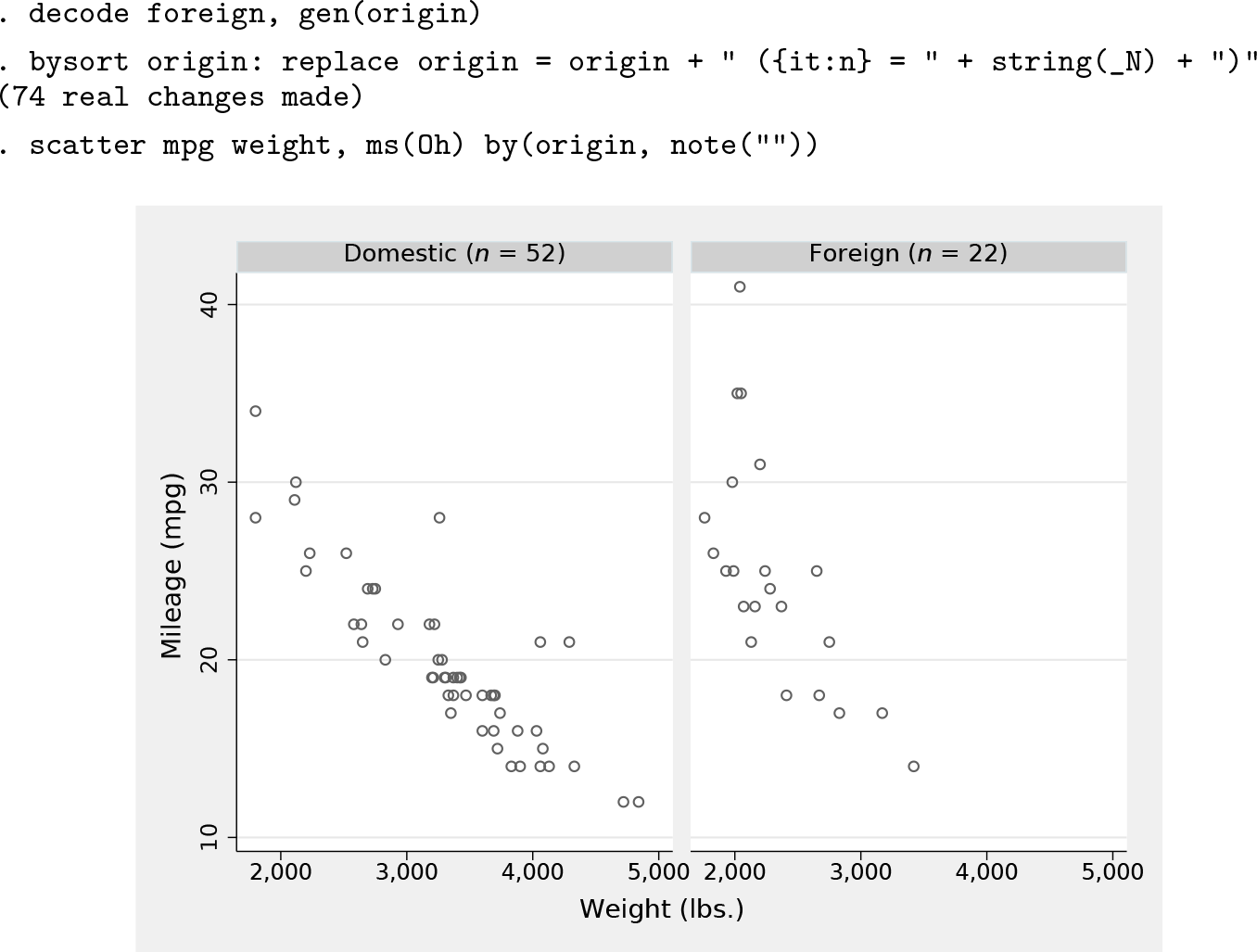
Once we have origin as a string variable, we can add extra text. The new variable can be used in the by() option. Figure 3 is the result.

Figure 3.1

The text for the by() variable has been enhanced for this display. The result appears automatically as subtitles.

That was suspiciously easy, so let’s close with a twistier example. Imagine evocative value labels for the prosaically numeric repair record variable rep78.

Alphabetically ordered, the labels would not match the underlying numeric order, even though they come awfully close. So decode would mangle the order, and the nettle to be grasped is to redefine the value labels. Here is how to do this through syntax. Loop over the possible values, look up the value label, count the number of values, and then apply an augmented label. The syntax for looking up value labels is documented at help macro. The result of a count is stored temporarily in r(N). Loops and local macros were introduced in a previous column (Cox 2020a).

Then, we can use the new labels in a graph (figure 4). Here we go beyond the main theme of a by: option to show that the technique of enhancing value labels has wider applications. Personal taste shows in putting the information for the numeric axis at the top whenever a graph has a tablelike flavor (Cox 2012).

Figure 3.2.

Dot chart for mean mpg by repair record, with whimsical value labels and a reminder of the number of observations.

You might prefer to do that interactively, say, by using tabulate rep78 to get the frequencies and then typing in revised text in the Variables Manager varm. As before, the syntax is simple because there are no missing values of mpg.

References

1.
ClevelandW. S.1994. The Elements of Graphing Data. Rev. ed. SummitNJ: Hobart.
CoxN. J.2020b. Stata tip 139: The by() option of graph can work better than graph combine. Stata Journal20: 1016–1027. https://doi.org/10.1177/1536867X20976341.