Review of Michael N. Mitchell’s Interpreting and Visualizing Regression Models Using Stata,Second Edition

Abstract

In this article, we review Interpreting and Visualizing Regression Models Using Stata, Second Edition, by Michael N. Mitchell (2021, Stata Press).

1 Introduction

In 2016, for the first time, the second author taught a 12-week master’s-level statistics course for psychology students, and he used the first (2012) edition of Michael N. Mitchell’s Interpreting and Visualizing Regression Models Using Stata (IVRMUS-1) as the primary textbook. Because many students would likely use some type of regression modeling for their thesis project, the topics covered in IVRMUS-1 seemed to be a good fit for the course, providing students with a practical grounding in ordinary least-squares (OLS) linear models but also introducing them to some other types of models. In 2019, the first author was a student in that same course. We hope that by collaborating on this book review, we will manage to bring not just an instructor’s perspective, which is typical in such reviews, but also a student’s perspective, which we believe is valuable but less often considered.

2 Content

Mitchell opens the preface to the second edition of IVRMUS (which we denote IVRMUS-2) by commenting on some changes that arose from his use of Stata 16.1 in the second edition; he used Stata 12.1 in the first edition. He notes, for example, that when results for the levels of a factor variable are displayed, value labels are shown rather than values (for example, Unmarried versus Married rather than 1 versus 2). He also comments on the availability of new small-sample options for the mixed and contrast commands. He then reaffirms his motivation for writing the book:

As with the first edition, I hope the examples shown in this book help you understand the results of your regression models so you can interpret and present them with clarity and confidence.

In the introductory chapter that follows, Mitchell draws a distinction between the teaching approach in his book (he calls it a “discovery learning perspective”) and the way one should approach research. He specifically cautions readers that his approach might seem to endorse some “bad research habits”: 1) letting the pattern of the data guide the analysis; 2) dissecting the results in every possible way; and 3) having no concern for the overall type I error rate. (We shall say more later about these bad habits.)

Mitchell then describes the datasets that he used, especially the General Social Survey dataset, which he uses most frequently. Four variables appear most often in his examples: income, age, years of education, and gender. For each variable, he gives some insight into analytic choices made in later chapters (for example, including the option vce(robust) when using regress to model income because income is positively skewed). Four other types of datasets are used in the book (for example, the school datasets used to illustrate multilevel modeling).

Although Mitchell does not say so explicitly in his preface, the commands margins, marginsplot, and contrast are once again the real workhorses of IVRMUS-2, as they were in the first edition. The pwcompare and lincom commands play important secondary roles.

2.1 Part I: OLS models with continuous explanatory variables

Chapter 2 introduces readers to the margins and marginsplot commands in the context of the simple linear regression model. It then moves on to multiple linear regression models and includes examples showing how to get fitted values of Y (or adjusted means, as Mitchell calls them) at selected values of the explanatory variables. It also discusses various ways to check for nonlinearity, both graphically and analytically.

Chapter 3 shows readers how to include quadratic and cubic terms in OLS models and also introduces the fp prefix command for fitting fractional polynomial models. On the latter, Mitchell cautions readers to be wary of overfitting whenever they “let the computer perform automatic modeling” and recommends some kind of cross-validation in that case.

Chapter 4 introduces the mkspline command and piecewise regression models. It includes examples of the following types of piecewise models:

One known knot, no jump

Two known knots, no jumps

One known knot with a jump

Two known knots with two jumps

One unknown knot

Multiple unknown knots

Mitchell also introduces the lincom command in this chapter, showing how it can be used to estimate the change in slope at a knot (when individual slope coding is used) or to estimate the slope within a certain segment (if change in slope coding is used). He concludes the chapter by showing how to use margins and marginsplot with piecewise models and offers some suggestions for automating graphs of piecewise models.

Chapters 5 and 6 discuss two-way and three-way interactions involving continuous (or quantitative) variables only. Examples of the following types of interactions are included:

Linear × linear

Linear × quadratic

Linear × linear × linear

In these chapters, Mitchell also shows readers how they can easily obtain simple slopes for one variable at selected values of another variable (or at selected combinations of values in higher-order interactions) via the dydx() option for margins.

2.2 Part II: OLS models with categorical explanatory variables

In part II, the emphasis is on interpreting and visualizing results pertaining to categorical explanatory variables. However, many of the models fit do include continuous covariates—age, for example.

Chapter 7 starts with an unpaired t test but then quickly moves on to fit a model including two categorical explanatory variables (marital status and gender) and one continuous covariate (age) by using the anova command. Mitchell issues a basic margins command to show adjusted means for the five marital status categories. He follows that with another margins command using the r. contrast operator to produce all pairwise contrasts with the reference group, married.

Next he introduces the contrast command and shows how to generate several kinds of contrast:

Reference group contrasts (r. operator)

Grand mean contrasts (g. operator)

Adjacent contrasts (a. operator)

Reverse-adjacent contrasts (ar. operator)

Helmert contrasts (h. operator)

Reverse Helmert contrasts (j. operator)

Polynomial contrasts (p. and q. operators)

Custom contrasts

Weighted contrasts (gw., hw., jw., pw., and qw. operators)

The chapter ends with examples of pairwise comparisons obtained via pwcompare and with a section showing how one can fit the same OLS model by using either anova or regress.

Table 7.1 is a highlight of chapter 7. It lists all the contrast operators along with descriptions of what they do and the chapter sections in which they are illustrated. The second author of this review has bookmarked that page.

Chapter 8 examines models with 2×2, 2×3, and 3×3 interactions. For 2×2 models, Mitchell shows how to estimate the “size” of the interaction (that is, the difference in differences). For the models with 2 × 3 and 3 × 3 interactions, he shows how to examine simple effects, simple contrasts, partial interactions, and interaction contrasts. The initial examples have balanced designs, but Mitchell also discusses unbalanced designs in section 8.5. In section 8.6, he shows that the 2 × 2 ANOVA fit earlier in the chapter using anova can also be fit using regress. But he takes pains to explain to readers that the coefficients in the regress output that look like main effects of the two variables are actually simple main effects.

Chapter 9 examines 2×2×2, 2×2×3, and 3×3×3 models. It shows readers how to examine simple interactions, simple effects, simple contrasts, partial interactions, and interaction contrasts.

2.3 Part III: OLS models with both continuous and categorical explanatory variables

Chapter 10 describes linear by categorical interactions. It starts with a first-order-effects-only model in which the two focal variables are age and college graduation status (1 = yes, 0 = no). Mitchell demonstrates how margins can be used to obtain both adjusted and unadjusted means, the latter by using the over() option. Next this model is extended to include the interaction between the two focal predictors. Mitchell uses margins to obtain adjusted means at selected values, as well as simple slopes for the continuous variable at each level of the categorical variable. He shows how to examine simple contrasts by adding the contrast option to the margins command. He then extends these methods to interactions between a continuous and three-level categorical variable, including testing the overall interaction size by using the contrast command and exploring partial interactions.

Chapter 11 builds on chapters 3 and 10 to explore polynomial by categorical interactions. Mitchell illustrates a quadratic by two-level categorical variable interaction, a quadratic by three-level categorical variable interaction, and a cubic by two-level categorical variable interaction. In each section, he begins by using a lowess smoother to determine whether such an interaction is needed. He again uses contrast, margins, and marginsplot to test the overall interaction effect, compute and compare the adjusted means, and plot the contrasts.

Chapter 12 expands on chapters 4 and 10 to explore piecewise by categorical interactions. Mitchell gives one-knot and two-knot examples, using gender as the categorical variable. He shows how to make various comparisons, including between- and within-gender comparisons of slopes, changes in slopes at knots, and changes in intercepts at knots. Adjusted means are also computed, with suggestions for automating graphs. (Here readers should see chapter 4 for a reminder of why the marginsplot command is not applicable.) Mitchell then devotes a section to four different coding schemes for these models.

Chapter 13 discusses two kinds of three-way interactions: linear by linear by categorical and linear by quadratic by categorical. Mitchell initially approaches these complex interactions by fitting separate regression models for each level of the categorical variable using by, sort:. He then bridges this with the full regression model with the complete interaction term. He shows how to visualize and interpret the interaction by using margins, contrast, and marginsplot.

Chapter 14 examines categorical by categorical by continuous interactions. Here Mitchell interprets these interactions in terms of how the slope of the continuous variable varies, depending on the interaction of the two categorical variables. He forms contrasts with respect to this slope, examining simple effects, simple contrasts, and partial interactions.

2.4 Part IV: Some other types of models

In part IV, Mitchell introduces multilevel models, logistic regression, Poisson regression, and use of the svy prefix command to analyze complex survey data.

Chapter 15 covers multilevel models, wherein Mitchell introduces the mixed command. Mitchell’s primary focus is showing how cross-level interactions can be interpreted in the same way as the interactions covered in earlier chapters. An example is given for each of the following interactions:

Continuous by continuous

Continuous (level-1 variable) by categorical (level-2 variable)

Categorical (level-1 variable) by continuous (level-2 variable)

Categorical by categorical

Chapter 16 covers longitudinal models with time as a continuous predictor. Mitchell acknowledges that several different approaches can be used to analyze longitudinal data, but as in chapter 15 he focuses strictly on multilevel models. He uses the xtreg command to fit a random-intercept model with time as the sole predictor, and then he uses the mixed command to fit a random-coefficients model. He also discusses modeling time in a piecewise manner whenever a baseline period precedes a treatment period. A focus of this chapter is examining cross-level interactions between treatment group and time, both linearly and piecewise. For the piecewise models, he shows how to compare a variety of values as a function of the treatment group, such as baseline slopes, jumps in outcome, changes in slope at the knot, and predicted means at different times.

Chapter 17 covers multilevel models for longitudinal data with time as a categorical variable. Mitchell includes examples of time as the sole fixed effect, interacted with a two-level group variable, and interacted with a three-level group variable. The interactions are interpreted using techniques similar to those in earlier chapters on categorical interactions, such as partial interactions. Mitchell also discusses how to choose a residual covariance structure. New to this edition, the last section covers adjustment for small samples via the dfmethod() and small options. For dfmethod(), one can choose between the Kenward–Roger and Satterthwaite methods.

Chapter 18 covers nonlinear models, including logistic, multinomial logistic, ordinal logistic, and Poisson models. Mitchell shows how the contrast, pwcompare, margins, and marginsplot commands apply to these cases. He also shows how to interpret 2 × 2 interactions for binomial logistic regression and how to fit a piecewise model with a binary outcome. Throughout this chapter, the natural metric of the model, such as log odds, is compared with those of linear models. Other metrics like probabilities can be chosen to ease interpretation, but they may be differentially affected by covariate values.

Chapter 19 covers complex survey data. Using the svy prefix, Mitchell shows how margins, contrast, and pwcompare can be used to compute estimates adjusted for the survey design.

2.5 Part V: The appendices

Five appendices cover additional options, features, and ways to customize the output of focal commands covered in the book, including estimation commands margins, contrast, pwcompare, and marginsplot.

3 Suggestions for the future

We believe that Mitchell has accomplished what he set out to do. He has provided many examples of typical regression problems that arise in research and shown how to visualize and interpret the results. Nevertheless, we do have some suggestions about how to improve any future edition, starting with some suggestions related to Stata code.

3.1 Stata code

Our first suggestion is addressed to the wider Stata community, not just to Mitchell. It is conventional in Stata documentation and in books about Stata to show code that is copied from the output window rather than to show the code such as one might see in a do-file. Mitchell follows this convention. In most cases, it does not cause undue problems, but consider this example on page 76:

In our experience, students who are new to Stata transcribe the code as shown and are perplexed when it does not run (given the line numbers that are included in the output). This problem could be avoided if Mitchell showed do-file code instead. Presumably, it looks something like this:

A second suggestion about code is to show readers how to use the /// continuation line indicator to split long commands over multiple lines. This would be particularly helpful for margins commands that have multiple at() clauses. On page 104, Mitchell shows this margins command:

We applaud the vertical alignment of the at() clauses. But readers who transcribe this command as shown will find that it does not work. We suggest that it be shown as follows:

Finally, we offer three more minor suggestions.

Include the clear option when opening data files.

Rather than writing (output omitted), use the quietly prefix command.

Show readers how to use the ciopts option to lighten the shaded confidence region when using the rarea option for marginsplot. We often include this option to make the shaded confidence region 40% as intense as the default setting: ciopts(color(*.4)).

3.2 The ibn and noconstant options

In chapters 11 to 13, Mitchell frequently uses the ibn prefix together with the option noconstant to obtain estimates of the intercept for each group. Although we prefer the more conventional approach of including a constant, we have no strong objection to Mitchell’s approach. However, we suggest spelling out to readers that his coding of the model results in an inflated R ² value that cannot be interpreted in the usual manner (that is, as the proportion of variance accounted for by the model). Mitchell skirts this issue in chapter 12 (section 12.4), where he shows four different coding schemes for the same model. Schemes 1 and 2 use ibn with noconstant, and schemes 3 and 4 use the more conventional approach (that is, they include the constant). But Mitchell uses the noheader option in all cases, thus obscuring the fact that the R ² values are inflated for schemes 1 and 2. We fear that in the absence of a comment about how ibn and noconstant affect R ², some readers who decide to use that coding scheme for their own data may inadvertently misinterpret the R ² value shown in their output.

Additionally, when ibn and noconstant are used throughout chapters 11–13, lowerorder terms appear to be missing from models that contain higher-order effects. We were puzzled by this at first, especially considering Mitchell’s warnings in earlier chapters (for example, chapter 3) to always include lower-order effects in models with interactions or polynomial terms. We reran some of the models in these later chapters, this time spelling out all lower-order terms and using the more conventional approach (that is, omitting ibn and noconstant). Here is our version of the example in section 13.2.2:

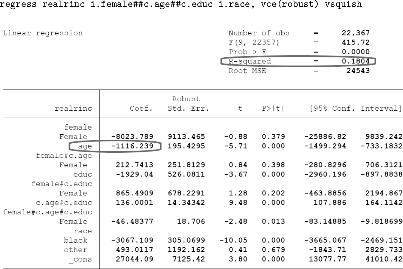
Compare this with Mitchell’s syntax and output for this example, repeated again here:

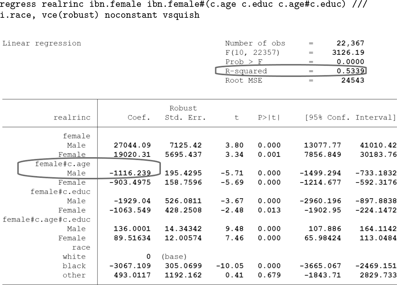
The lower-order effect for age does appear in Mitchell’s output, but it appears as the coefficient for Male under the female#c.age interaction. The same pattern occurs for other lower-order effects. This is because the lower-order effect of age is fit separately for male and female individuals. Essentially, all coefficients for lower-order terms will appear as coefficients for that term interacted with female in Mitchell’s model (as the base level). Thus, despite initial appearances, the lower-order effects are present in the model. Also note, as mentioned earlier, the inflated R ² in Mitchell’s model (R ² = 0.5339) compared with our model (R ² = 0.1804).

Overall, we would suggest comparing the output of both approaches. It may also be helpful to direct the reader to more information on how this coding affects the regression output (for example, Higbee [2009]). One quick sentence is devoted to explaining the function of ibn and noconstant in chapter 11, but its use throughout chapters 11–13 left us wondering why it was applied to those particular topics and in which other cases this coding scheme might be beneficial.

3.3 Terminology

Imagine a regression model with explanatory variables A and B, as well as their product, A × B. In such a model, Mitchell frequently refers to the coefficients for A and B as showing the main effects of those variables. We suggest that the term “main effect” should be reserved for ANOVA models, where the main effect of A is the effect of A when one collapses across the levels of B. In a regression model, on the other hand, the coefficient for A shows the simple effect of A when B = 0 (or its reference category if it is categorical). To be fair, Mitchell does explain this to readers. Nevertheless, in the context of regression models, we recommend describing the coefficients for A and B as the first-order effects of A and B to avoid this potential confusion.

We also suggest that it could be helpful if Mitchell briefly mentioned the terms “moderated multiple regression” and “effect modification”. The latter term is commonly used in epidemiology and medical research, and the former term is commonly used in psychology and related fields. This might seem like a trivial suggestion, but it is motivated by the fact that a psychology student who had worked through all the examples in IVRMUS-1 believed that he had never fit a moderated multiple regression model. It is not difficult to imagine that an epidemiology student might similarly believe that she had never fit a model that addressed a question about effect modification.

In the same vein, the literature on moderation would likely describe the approach Mitchell takes to interpreting interactions as the pick-a-point, simple-slopes, or spotlight-analysis approach and contrast it to other approaches like the Johnson–Neyman technique. As with the relationship between the terms “moderation” and “interaction”, it might be worthwhile to point out that many of the examples in IVRMUS-2 are analogous to the pick-a-point approach readers might see elsewhere. Additionally, Mitchell’s examples can be easily extended to create what otherwise might be referred to as a Johnson–Neyman plot. For instance, chapter 5 explores an interaction between age and education (both continuous variables). The code below computes and graphs the slope of education for every value of age, highlighting the regions where the slope is statistically significant.

3.4 Reminding the reader about bad research habits

We find the discussion of three bad research habits (section 1.1—Read me first) vitally important. Otherwise, one might blindly follow Mitchell’s examples in each chapter until some sort of statistical significance is achieved. Students still learning about best research practices might be more prone to this, and as such it would be a good idea to flag these habits throughout the text. One way this is already done is when Mitchell uses the mcompare() option within the pwcompare command, which adjusts for multiple comparisons and avoids bad research habit #3. This is briefly shown a couple of times; however, it would have been helpful to note how this option can also be used with the contrast command. To demonstrate avoiding bad research habits #1 and #2, it might be helpful to introduce an independent hypothesis before each new application of a command. Indeed, Mitchell sometimes does this, and there is only so much space. We simply fear that it might be easy to miss section 1.1.

3.5 Choosing values when probing interactions

When Mitchell interprets the effect of one predictor at specified values of another continuous predictor, the chosen values might seem randomly selected for the purpose of illustrating the example. Because readers might wonder which values to choose for their own analysis without conducting too many tests, it might be worth mentioning in IVRMUS-2 that often the choice of values to probe can be arbitrary, and this is sometimes noted as a drawback of the approach. Further, in these situations researchers sometimes choose to probe at the mean or certain percentiles (as recommended, for instance, by Hayes [2018], although sometimes no less arbitrary). Considering this, it would be worthwhile to use at(p( # )) for the at() option within the margins command more often because this is only done in chapter 18. This allows selecting values at certain percentiles.

3.6 Further explanations

Mitchell uses the mixed command for multilevel models throughout chapter 15, but he briefly switches to the xtreg command for one random-intercept multilevel model in chapter 16 without much introduction to the command. He then uses mixed again for the rest of the chapter. We think it would be helpful to add an explanation of why xtreg was appropriate for the example and how it compares with using the mixed command. Readers might not be familiar with xtreg and may wonder whether they should use xtreg or mixed for their multilevel model questions.

Finally, Mitchell uses the marginal option in his demonstration of various coding schemes in chapter 12.4. Because this is the first time the marginal option is used after chapter 4, we suggest adding a sentence on page 368 reminding readers that the marginal option is used for change in slope coding or referring them to chapter 4. This would help with understanding some of the differences between coding schemes.

3.7 Topics to add (or remove)

As noted above, we have used IVRMUS in a master’s-level statistics course for psychology students. In psychology and many other fields (for example, epidemiology), the hierarchical approach to building a regression model is quite popular. With that in mind, we believe that IVRMUS-2 would benefit from an example or two showing readers how to use the nestreg prefix command.

Mediation analysis is also increasingly common in both psychology and epidemiology. It would be good, therefore, to have a short chapter showing how one can fit regression models via sem and how one can use sem to fit mediation models. In our view, this would be more helpful to students and researchers in psychology than the current chapter 19 (on complex survey data).

4 Conclusion

As we noted earlier, Mitchell hoped that the examples shown in IVRMUS-2 would help readers understand the results of their own regression models and enable them to “interpret and present [their results] with clarity and confidence”. As our review shows, we do have some criticisms of the way Mitchell approached certain things, some suggestions for further aiding reader understanding, and some topics we would wish to see included in any future edition. But despite that, the second author has never regretted adopting IVRMUS-2 as the primary textbook for the master’s-level statistics course he recently taught for the fifth time. And the first author will continue to refer to IVRMUS-2 throughout her doctoral education and for years to come. In sum, we believe that Mitchell has achieved his objective admirably.

Supplemental Material

Supplemental Material, sj-zip-1-stj-10.1177_1536867X211063410 - Review of Michael N. Mitchell’s Interpreting and Visualizing Regression Models Using Stata, Second Edition

Supplemental Material, sj-zip-1-stj-10.1177_1536867X211063410 for Review of Michael N. Mitchell’s Interpreting and Visualizing Regression Models Using Stata, Second Edition by Angela MacIsaac and Bruce Weaver in The Stata Journal