On identification and estimation of Heckman models

Abstract

In this article, we present commands to enable fixing the value of the correlation between the unobservables in Heckman models. These commands can solve two practical issues. First, for situations in which a valid exclusion restriction is not available, these commands enable exploring how the results could be affected by sample-selection bias. Second, stepping through values of this correlation can verify whether the global maximum of the likelihood function has been found. We provide several commands to fit these and related models with a fixed value of the correlation between the unobservables.

1 Introduction

Heckman’s (1976, 1978) work on sample-selection and endogenous treatment models has been widely used in applied research. Convincing identification of these models requires an exclusion restriction (often referred to as an “instrument”), that is, a variable that affects selection or treatment but not the outcome directly. For many applications, a valid exclusion restriction is not available. Without a valid exclusion, identification of the model is only possible through the distributional assumptions placed on the model.

One approach to fitting a Heckman model without an exclusion restriction is to fix the value of the correlation between the unobservables in the selection and outcome equations (which we refer to as “rho”) at multiple plausible values. The idea is to treat rho as if it were unidentified rather than to identify it based on distributional assumptions. We can then see how the results are affected by the value of rho. As we discuss in the next section, we can think of rho as the degree of sample-selection bias. This approach was taken for endogenous treatment and sample-selection models by Altonji, Elder, and Taber (2005) and Chan and Cook (2020), respectively. Altonji, Elder, and Taber also propose using the correlation in observable characteristics to bound the possible values of the correlation in unobservable characteristics, which we do not discuss in this article.

We provide commands that enable fixing the value of rho and which are based on Altonji, Elder, and Taber (2005) and Chan and Cook (2020). This article’s commands have been used to address concerns about sample-selection bias when a valid exclusion is not available (as in Aobdia [2019]; Choudhary, Merkley, and Schipper [2019]; Downey, Bedard, and Boland [2020]; and Tran and Dinh [Forthcoming]).

Another benefit of fixing the value of rho is improved ease of maximizing the likelihood function. The likelihood functions for these models are known to be difficult to maximize. Zuehlke (2017) reports several instances in which authors have reported estimates that are not the global maximum of the likelihood function. The likelihood function is not globally concave, but if the value of rho is fixed, the likelihood is concave in the remaining parameters. Olsen (1982) suggests stepping through values of rho to find the global maximum of the likelihood function. Zuehlke notes that standard statistical software does not provide the option of maximizing the likelihood function in this manner. Rodemeier (2020) uses this article’s commands for this purpose.

We provide an example in section 4 of how to use these commands to step through values of rho to maximize the likelihood function. For this example, Stata’s heckman command does not provide the actual maximum-likelihood estimate unless the initial values are set to a neighborhood of the correct values.

The next section reviews Heckman’s sample-selection model and discusses the effect of fixing rho. Section 3 provides the syntax for the commands that we are introducing. In this section, we also discuss related models, including endogenous treatment models. Examples are provided in section 4. Section 5 concludes.

2 Heckman’s sample-selection model

When the observations used for a regression are nonrandomly selected, there is a concern that selection could affect the results. In the classic example of regressing education on wage for married women, there is a concern that the decision to work may be affected by both education and unobserved factors. ¹ The women with lower education who enter the workforce are those who expect higher wages. This self-selection can overstate the average wage for women with low education and bias the relationship between education and wage downward relative to the true causal effect.

We illustrate this effect in figure 1. Figure 1a presents a scatterplot and line of best fit for all observations (both observed and unobserved). A circle denotes that an instance was unobserved. Figure 1b removes the unobserved instances and adds a new line of best fit based on only the observed instances. The line of best fit from figure 1a is also presented for reference. Selection has decreased the slope of the line of best fit. An important point is that sample selection is a problem of bias, not of generalization to a wider population.

(b) Only selected observations

Figure 1.

Illustration of the effect of sample selection

The approach developed by Heckman (1976) to combat these concerns is to jointly estimate the selection and outcome processes. We begin by defining latent outcome and selection variables, $y_i^{*}$ and $s_i^{*}$ , as

$y_i^{*}=x_i\beta +{\epsilon }_i$

1

$s_i^{*}=z_i\gamma +u_i$

2

where

$\left(\begin{array}{c}{\epsilon }_i\\ u_i\end{array}\right)~N_2\left(\left[\begin{array}{l}0\hfill \\ 0\hfill \end{array}\right],\left[\begin{array}{cc}{\sigma }^2& \rho \sigma \\ \rho \sigma & 1\end{array}\right]\right)$

We refer to (1) as the “outcome equation” and (2) as the “selection equation”. We are assuming a linear relationship between the latent variables and the regressors x _i = (1, x _{1 ,i},…, x_k,i ) and z _i = (1, z _{1 ,i},…, z_r,i ). The coefficients β and γ are column vectors. The correlation between ε_i and u_i , denoted as ρ, is the same rho that was discussed in the introduction. For the remainder of this section, we will use the Greek letter ρ rather than writing out rho.

We observe an indicator for selection, s_i , and outcome, y_i , defined as

$\begin{array}{l}{s}_i=\{\begin{array}{cc}1& \text{ if }{s}_i^{*}>0\\ 0& \text{ otherwise }\end{array}\\ y_i=\{\begin{array}{cc}{y}_i^{*}& \text{if }{s}_i=1\\ 0& \text{if }{s}_i=0 \end{array}\end{array}$

3

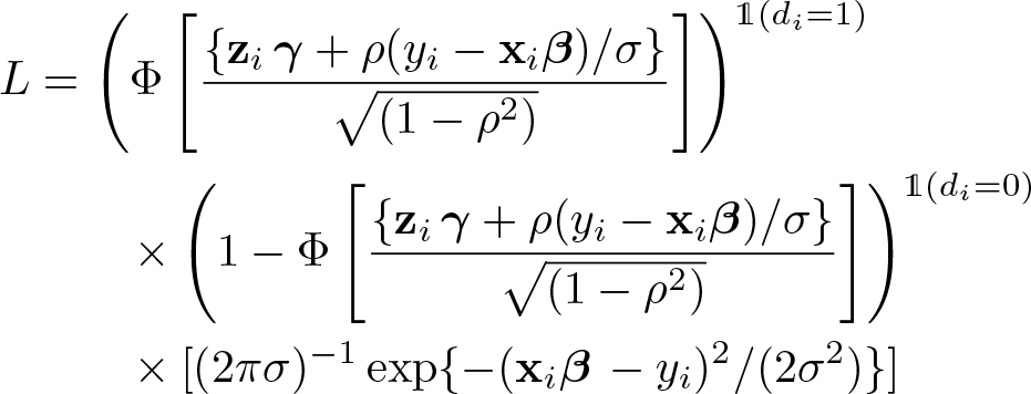
The value of y_i when s_i = 0 is arbitrary and unimportant because these values will not be used for estimation. The parameters of interest (β, γ, σ, and ρ) can be estimated by maximizing the likelihood function

$\begin{array}{c}L={\displaystyle \prod _i\Phi }{\left\{-\left(\gamma z_i\right)\right\}}^{1\left(s_i=0\right)}\times {\left(\Phi \left[\frac{\left\{\gamma z_i+\rho \left(y_i-\beta x_i\right)/\sigma \right\}}{\sqrt{\left(1-{\rho }^2\right)}}\right]\right)}^{1\left(s_i=1\right)}\\ \times {\left[{(2\pi \sigma )}^{-1}\exp \left\{-{\left(\beta x_i-y_i\right)}^2/\left(2{\sigma }^2\right)\right\}\right]}^{1\left(s_i=1\right)}\end{array}$

where φ(·) and Φ(·) are the standard normal density and distribution functions and 1(A) is the indicator function, which takes a value of 1 if the event A is true and a value of 0 otherwise. Stata’s heckman command performs this maximum likelihood estimation as well as the popular “two-step” estimator of this model. We do not discuss the two-step estimator here, because our approach of fixing the value of ρ is less straightforward with the two-step estimator.

2.1 Fixing the value of ρ

For the observed data, the expected value of the outcome is

$\begin{array}{c}E\left(y_i|x_i,s_i=1\right)=x_i\beta +E\left({\epsilon }_i|s_i=1\right)\\ =x_i\beta +\rho \sigma \varphi \left(z_i\gamma \right)/\Phi \left(z_i\gamma \right)\end{array}$

The term ɸ(·)/Φ(·), known as the inverse Mills ratio, follows from the bivariate normality assumption that was placed on ε_i and u_i . An insight from Heckman (1979) is that sample-selection bias can be thought of as an omitted-variable bias, where the omitted variable is the inverse Mills ratio. Naively regressing y_i on x _i results in a bias of

$\rho \hspace{0.17em}\sigma {\{\text{Var}(x)\}}^{-}{ }^1\text{Cov}\{x,ɸ(z\gamma )/\Phi (z\gamma )\}$

where x and z are the usual matrices of regressors. This bias is increasing in the value of ρ. When ρ equals 0, there is no bias for the naive estimate. It is in this sense that we can think of ρ as the degree of sample-selection bias.

We first discuss the role of fixing the value of ρ on identification, and then we turn to the problem of maximizing the likelihood function. For discussing identification, it is useful to contrast this model to semiparametric sample-selection models. The inconsistency of Heckman’s estimator in the presence of nonnormal errors (as shown by Arabmazar and Schmidt [1982] and Robinson [1982]) inspired the creation of several semiparametric estimators. These estimators relax the bivariate normality assumption to accommodate a broader class of bivariate distributions. While Heckman’s parametric estimator is identified even when x and z contain the same variables (that is, there is no exclusion restriction), these semiparametric estimators require an exclusion restriction for identification. A common finding in Monte Carlo experiments is that Heckman’s estimator performs surprisingly well with nonnormal errors as long as there is a valid exclusion restriction (see, for example, Cook and Siddiqui [2020]). This finding has contributed to the widespread use of Heckman’s model when there is a valid exclusion restriction.

To be clear, throughout this article, we refer to the exclusion restriction as “valid”, meaning that the excluded variable or variables do not affect the outcome directly. It may be tempting to simply omit a variable from the outcome equation so that the model has an excluded variable. This approach, however, can result in estimates that are worse than those obtained by ordinary least squares (Wolfolds and Siegel 2019). ²

The assumption that the unobservables follow a bivariate normal distribution, which is required for identification without an exclusion restriction, is generally untestable without a valid exclusion restriction. To identify the distribution of ε_i , we need to identify β. The coefficients β could be estimated using a semiparametric estimator, but these estimators require a valid exclusion restriction.

Regarding finding the maximum of the likelihood function, once the value of ρ is fixed, Stata can easily find the values of the other parameters that maximize the likelihood function. If we step through different values of ρ, we can see where the likelihood function is maximized. This can be used to verify that the results returned by heckman are the true maximum and to set the initial values if Stata is not returning the global maximum.

Having discussed both a sensitivity test and a method for finding the maximum of the likelihood function, there are two points that should be made explicit. First, one should not step through values of rho to maximize the likelihood function when a valid exclusion restriction is not available. While exploring how the results differ for different values of ρ illustrates how sensitive the results are to the degree of sample-selection bias, this procedure cannot be used to reliably estimate the value of ρ when there is no exclusion restriction. Second, for situations in which an exclusion restriction is available, to get the correct standard errors and p-values, Stata’s heckman command should be called with initial values set near the global maximum. The standard errors and p-values that are found with a fixed value of ρ may differ from those found without the value of ρ fixed.

3 Syntax

This section provides the syntax for the eight commands that we are introducing: heckman_fixedrho, heckman_scanrho, heckprobit_fixedrho, heckprobit_scanrho, etregress_fixedrho, etregress_scanrho, biprobit_fixedrho, and biprobit_scanrho. Each is named after the command upon which it was based with the added suffix fixedrho or scanrho. An important difference between these commands and their built-in counterparts is that these commands do not offer all the options that the other commands do. There are also some slight syntax differences that we highlight below.

In this section, we also provide a brief overview about the relevant models that are fit with the Stata commands heckprobit, etregress, and biprobit. References are provided for any reader seeking more details.

3.1 Heckman’s sample-selection model

Syntax for heckman_fixedrho

We now present the syntax for the first command, heckman_fixedrho, which is for setting the value of rho.

heckman_fixedrho depvar [indepvars] [if] [in] , select( depvar_s = varlist s [, offset( varname ) noconstant ]) rho( # ) [vce( vcetype ) level( # ) maximize_options ]

Options for heckman_fixedrho

select( depvar_s = varlist_s [, offset( varname ) noconstant]) specifies the selection equation. select() is required.

depvar_s should be coded as 0 or 1, with 0 indicating an observation not selected and 1 indicating a selected observation.

rho( # ) specifies the correlation between the unobservables in the selection and outcome equations. rho() is required and must take a value between −1 and 1.

vce( vcetype ) specifies the type of standard errors to be used for the estimates. vcetype may be oim, robust, cluster( clustvar ), opg, bootstrap, or jackknife.

level( # ) sets the confidence level. The default is level(95) or as set by set level.

maximize_options control the maximization process. Options include difficult, [no]log, trace, gradient, showstep, hessian, showtolerance, tolerance( # ), ltolerance( # ), nrtolerance( # ), and nonrtolerance. These options are seldom used.

Syntax for heckman_scanrho

We now present the syntax for the next command, heckman_scanrho, which is for scanning through values of ρ.

heckman_scanrho depvar [indepvars] [if] [in] , select( depvar_s = varlist_s [, offset( varname ) noconstant]) [minrho( # ) maxrho( # ) step( # ) vce( vcetype ) level( # ) nograph maximize_options]

Options for heckman_scanrho

select( depvar_s = varlist_s [, offset( varname ) noconstant]) specifies the selection equation. select() is required.

depvar_s should be coded as 0 or 1, with 0 indicating an observation not selected and 1 indicating a selected observation.

minrho( # ) specifies the minimum value of correlation between the unobservables in the selection and outcome equations to be considered. It must take a value between −1 and 1. Note that convergence may be difficult at values of −1 and 1. The default is minrho(-0.9).

maxrho( # ) specifies the maximum value of correlation between the unobservables in the selection and outcome equations to be considered. It must take a value between −1 and 1. Note that convergence may be difficult at values of −1 and 1. The default is maxrho(0.9).

step( # ) specifies the size of the step to use when scanning over values of correlation. This procedure will take a long time to run when the step size is small. The default is step(0.01).

vce( vcetype ) specifies the type of standard errors to be used for the estimates. vcetype may be oim, robust, cluster( clustvar ), opg, bootstrap, or jackknife.

level( # ) sets the confidence level. The default is level(95) or as set by set level.

nograph suppresses the graphical output.

maximize_options control the maximization process. Options include difficult, [no]log, trace, gradient, showstep, hessian, showtolerance, tolerance( # ), ltolerance( # ), nrtolerance( # ), and nonrtolerance. These options are seldom used.

We now turn to discussing related models that can be thought of as extensions to the sample-selection model discussed above. Our discussion of each is brief, but we provide references for the reader wishing to gain more information.

3.2 Bivariate probit with sample selection

For an outcome that is binary instead of continuous, it is straightforward to extend the model above (as was done by Van de Ven and Van Praag [1981]). We maintain the latent variables in (1) and (2) and the selection indicator in (3):

$\begin{array}{l}{y}_i^{*}=x_i\beta +{\epsilon }_i\\ s_i^{*}=z_i\gamma +u_i\\ s_i=\{\begin{array}{ll}1\hfill & \text{ if }{s}_i^{*}>0\hfill \\ 0\hfill & \text{ otherwise }\hfill \end{array}\end{array}$

But now we define the observed outcome as

$y_i=\{\begin{array}{ll}1\hfill & \text{ if }{y}_i^{*}>0\text{ and }{s}_i=1\hfill \\ 0\hfill & \text{ if }{y}_i^{*}\le 0\text{ and }{s}_i=1\hfill \\ 0\hfill & \text{ if }{s}_i=0\hfill \end{array}$

The likelihood function is

$L={\displaystyle \prod _i{\Phi }_2}{\left(z_i\gamma ,x_i\beta ;\rho \right)}^{1\left(y_i=1\right)}\times {\Phi }_2{\left(z_i\gamma ,-x_i\beta ;-\rho \right)}^{1\left(y_i=0,s_i=1\right)}\times \Phi {\left(-z_i\gamma \right)}^{1\left(s_i=0\right)}$

Syntax for heckprobit_fixedrho

In Stata, the command heckprobit fits this model. We now present the syntax for heckprobit_fixedrho, which can be used to set the value of ρ in this model.

heckprobit_fixedrho depvar [indepvars] [if] [in], select( depvar_s = varlist_s [, offset( varname ) noconstant]) rho( # ) [vce( vcetype ) level( # ) maximize_options]

Options for heckprobit_fixedrho

select( depvar_s = varlist_s [, offset( varname ) noconstant]) specifies the selection equation. select() is required.

depvar_s should be coded as 0 or 1, with 0 indicating an observation not selected and 1 indicating a selected observation.

rho( # ) specifies the correlation between the unobservables in the selection and outcome equations. rho() is required and must take a value between −1 and 1.

vce( vcetype ) specifies the type of standard errors to be used for the estimates. vcetype may be oim, robust, cluster( clustvar ), opg, bootstrap, or jackknife.

level( # ) sets the confidence level. The default is level(95) or as set by set level.

maximize_options control the maximization process. Options include difficult, [no]log, trace, gradient, showstep, hessian, showtolerance, tolerance( # ), ltolerance( # ), nrtolerance( # ), and nonrtolerance. These options are seldom used.

Syntax for heckprobit_scanrho

We now present heckprobit_scanrho, which can be used to scan through values of ρ.

heckprobit_scanrho depvar [indepvars] [if] [in] , select( depvar_s = varlist_s [, offset( varname ) noconstant]) [minrho( # ) maxrho( # ) step( # ) vce( vcetype ) level( # ) nograph maximize_options]

Options for heckprobit_scanrho

select( depvar_s = varlist_s [, offset( varname ) noconstant]) specifies the selection equation. select() is required.

depvar_s should be coded as 0 or 1, with 0 indicating an observation not selected and 1 indicating a selected observation.

minrho( # ) specifies the minimum value of correlation between the unobservables in the selection and outcome equations to be considered. It must take a value between −1 and 1. Note that convergence may be difficult at values of −1 and 1. The default is minrho(-0.9).

maxrho( # ) specifies the maximum value of correlation between the unobservables in the selection and outcome equations to be considered. It must take a value between −1 and 1. Note that convergence may be difficult at values of −1 and 1. The default is maxrho(0.9).

step( # ) specifies the size of the step to use when scanning over values of correlation. This procedure will take a long time to run when the step size is small. The default is step(0.01).

vce( vcetype ) specifies the type of standard errors to be used for the estimates. vcetype may be oim, robust, cluster( clustvar ), opg, bootstrap, or jackknife.

level( # ) sets the confidence level. The default is level(95) or as set by set level.

nograph suppresses the graphical output.

maximize_options control the maximization process. Options include difficult, [no]log, trace, gradient, showstep, hessian, showtolerance, tolerance( # ), ltolerance( # ), nrtolerance( # ), and nonrtolerance. These options are seldom used.

3.3 Endogenous binary regressors

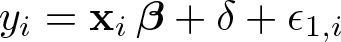
Heckman (1978) tackles the problem of endogenous binary regressors using a similar strategy as that of sample selection. The problem is stated in terms of the observed variables:

$y_i=x_i\beta +d_i\delta +{\epsilon }_i$

4

$d_i=\{\begin{array}{ll}1\hfill & \text{ if }{z}_i\gamma +u_i>0\hfill \\ 0\hfill & \text{ otherwise }\hfill \end{array}$

5

where

$\left(\begin{array}{c}{\epsilon }_i\\ u_i\end{array}\right) ~N_2\left(\left[\begin{array}{l}0\hfill \\ 0\hfill \end{array}\right],\left[\begin{array}{cc}{\sigma }^2& \rho \sigma \\ \rho \sigma & 1\end{array}\right]\right)$

The likelihood function can be expressed as

$\begin{array}{c}L=(\Phi {\left[\frac{\left\{z_i\gamma +\rho \left(y_i-x_i\beta \right)/\sigma \right\}}{\sqrt{\left(1-{\rho }^2\right)}}\right])}^{1\left(d_i=1\right)}\\ \times {\left(1-\Phi \left[\frac{\left\{z_i\gamma +\rho \left(y_i-x_i\beta \right)/\sigma \right\}}{\sqrt{\left(1-{\rho }^2\right)}}\right]\right)}^{1\left(d_i=0\right)}\\ \times \left[{(2\pi \sigma )}^{-1}\exp \left\{-{\left(x_i\beta -y_i\right)}^2/\left(2{\sigma }^2\right)\right\}\right]\end{array}$

This problem can also be expressed in the context of the Neyman–Rubin potential-outcomes framework.

In the potential-outcomes framework, those receiving a treatment have the outcome

$y_i=x_i\beta +\delta +{\epsilon }_{1,i}$

whereas those not receiving the treatment have the outcome

$y_i=x_i\beta +{\epsilon }_{0,i}$

The parameter δ is the average treatment effect after removing the confounding effects of treatment assignment, which Heckman (1990, 314) calls the “experimental treatment effect”. In this potential-outcomes framework, the outcome and treatment can still be expressed as in (4) and (5), but the error term in (4) is defined as

${\epsilon }_i=d_i{\epsilon }_{1,i}+ (1-d_i){\epsilon }_{0,i}$

The variances of ∊ _{1 ,i} and ∊ _{0 ,i} and their correlations with u_i may differ. In Stata, the command etregress can fit this model with and without allowing for potentially different variances and correlations for the unobservables for the treated and untreated.

Syntax for etregress_fixedrho

The syntax for our command etregress_fixedrho is as follows:

etregress_fixedrho depvar [indepvars] [if] [in], treat( depvar_s = varlist_s ) rho( # ) [ poutcomes vce( vcetype ) level( # ) maximize_options]

Options for etregress_fixedrho

treat( depvar_s = varlist_s ) specifies the treatment equation. treat() is required.

depvar_s should be coded as 0 or 1, with 0 indicating an observation not selected and 1 indicating a selected observation.

rho( # ) specifies the correlation between the unobservables in the selection and outcome equations. rho() is required and must take a value between −1 and 1.

poutcomes uses a potential-outcomes model with separate treatment and control group variances.

vce( vcetype ) specifies the type of standard errors to be used for the estimates. vcetype may be oim, robust, cluster( clustvar ), opg, bootstrap, or jackknife.

level( # ) sets the confidence level. The default is level(95) or as set by set level.

maximize_options control the maximization process. Options include difficult, [no]log, trace, gradient, showstep, hessian, showtolerance, tolerance( # ), ltolerance( # ), nrtolerance( # ), and nonrtolerance. These options are seldom used.

Syntax for etregress_scanrho

The syntax for etregress_scanrho follows. Note that the potential-outcomes option is not allowed.

etregress_scanrho depvar [indepvars] [if] [in], treat( depvar_s = varlist_s ) [minrho( # ) maxrho( # ) step( # ) vce( vcetype ) level( # ) nograph maximize_options]

Options for etregress_scanrho

treat( depvar_s = varlist_s ) specifies the treatment equation. treat() is required.

depvar_s should be coded as 0 or 1, with 0 indicating an observation not selected and 1 indicating a selected observation.

minrho( # ) specifies the minimum value of correlation between the unobservables in the selection and outcome equations to be considered. It must take a value between −1 and 1. Note that convergence may be difficult at values of −1 and 1. The default is minrho(-0.9).

maxrho( # ) specifies the maximum value of correlation between the unobservables in the selection and outcome equations to be considered. It must take a value between −1 and 1. Note that convergence may be difficult at values of −1 and 1. The default is maxrho(0.9).

step( # ) specifies the size of the step to use when scanning over values of correlation. This procedure will take a long time to run when the step size is small. The default is step(0.01).

vce( vcetype ) specifies the type of standard errors to be used for the estimates. vcetype may be oim, robust, cluster( clustvar ), opg, bootstrap, or jackknife.

level( # ) sets the confidence level. The default is level(95) or as set by set level.

nograph suppresses the graphical output.

maximize_options control the maximization process. Options include difficult, [no]log, trace, gradient, showstep, hessian, showtolerance, tolerance( # ), ltolerance( # ), nrtolerance( # ), and nonrtolerance. These options are seldom used.

3.4 Bivariate probit

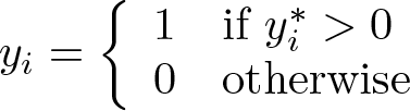
This next model (known as a recursive simultaneous-equation model) is not actually an extension of Heckman but was developed independently of Heckman’s work (see Maddala and Lee [1976]). We include this model in our discussion because it bears a similarity to the aforementioned models. We begin with (4) and (5) but now interpret (4) as a latent variable:

$\begin{array}{l}{y}_i^{*}=x_i\beta +d_i\delta +{\epsilon }_i\\ d_i=\{\begin{array}{ll}1\hfill & \text{ if }{z}_i\gamma +u_i>0\hfill \\ 0\hfill & \text{ otherwise }\hfill \end{array}\end{array}$

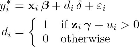
We denote the latent outcome as $y_i^{*}$ rather than y_i to emphasize that it is not directly observed. The unobservables ε_i and u_i still follow bivariate normal distribution, but now the variance of ε_i is set to 1:

$\left(\begin{array}{c}{\epsilon }_i\\ u_i\end{array}\right)~N_2\left(\left[\begin{array}{l}0\hfill \\ 0\hfill \end{array}\right],\left[\begin{array}{ll}1\hfill & \rho \hfill \\ \rho \hfill & 1\hfill \end{array}\right]\right)$

The econometrician observes d_i and the outcome

$y_i=\{\begin{array}{ll}1\hfill & \text{ if }{y}_i^{*}>0\hfill \\ 0\hfill & \text{ otherwise }\hfill \end{array}$

Syntax for biprobit_fixedrho

In Stata, the command biprobit can be used to fit this model. To maintain a syntax similar to our other commands (for example, heckman_fixedrho), which function similarly, the syntax for our command biprobit_fixedrho differs from biprobit.

biprobit_fixedrho depvar [indepvars] [if] [in] , eq2( depvar_s = varlist_s ) rho( # ) [vce( vcetype ) level( # ) maximize_options]

Options for biprobit_fixedrho

eq2( depvar_s = varlist_s ) specifies the second equation. eq2() is required.

depvar_s should be coded as 0 or 1, with 0 indicating an observation not selected and 1 indicating a selected observation.

rho( # ) specifies the correlation between the unobservables in the selection and outcome

equations. rho() is required and must take a value between −1 and 1.

vce( vcetype ) specifies the type of standard errors to be used for the estimates. vcetype may be oim, robust, cluster( clustvar ), opg, bootstrap, or jackknife.

level( # ) sets the confidence level. The default is level(95) or as set by set level.

maximize_options control the maximization process. Options include difficult, [no]log, trace, gradient, showstep, hessian, showtolerance, tolerance( # ), ltolerance( # ), nrtolerance( # ), and nonrtolerance. These options are seldom used.

Syntax for biprobit_scanrho

Finally, we provide the syntax for biprobit_scanrho.

biprobit_scanrho depvar [indepvars] [if] [in] , eq2( depvar_s = varlist_s ) [minrho( # ) maxrho( # ) step( # ) vce( vcetype ) level( # ) nograph maximize_options]

Options for biprobit_scanrho

eq2( depvar_s = varlist_s ) specifies the second equation. eq2() is required.

depvar_s should be coded as 0 or 1, with 0 indicating an observation not selected and 1 indicating a selected observation.

minrho( # ) specifies the minimum value of correlation between the unobservables in the selection and outcome equations to be considered. It must take a value between −1 and 1. Note that convergence may be difficult at values of −1 and 1. The default is minrho(-0.9).

maxrho( # ) specifies the maximum value of correlation between the unobservables in the selection and outcome equations to be considered. It must take a value between −1 and 1. Note that convergence may be difficult at values of −1 and 1. The default is maxrho(0.9).

step( # ) specifies the size of the step to use when scanning over values of correlation. This procedure will take a long time to run when the step size is small. The default is step(0.01).

vce( vcetype ) specifies the type of standard errors to be used for the estimates. vcetype may be oim, robust, cluster( clustvar ), opg, bootstrap, or jackknife.

level( # ) sets the confidence level. The default is level(95) or as set by set level.

nograph suppresses the graphical output.

maximize_options control the maximization process. Options include difficult, [no]log, trace, gradient, showstep, hessian, showtolerance, tolerance( # ), ltolerance( # ), nrtolerance( # ), and nonrtolerance. These options are seldom used.

4 Examples

The help file for each command provides some examples of the syntax. In this section, we discuss the application of these commands.

Identification without an exclusion restriction

Our first example considers bounding the potential effect of sample selection when we do not have a valid exclusion restriction. We use Mroz’s (1987) well-known dataset of married women’s wages in the 1970s. Some of the women in this dataset do not work, and thus there is no observed wage for these women. Our interest is in the effect of education on wage.

We can load this dataset by typing

use http://fmwww.bc.edu/ec-p/data/wooldridge/mroz

Suppose that we want to regress log wage (lwage) on years of education (educ), experience (exper), and experience squared (expersq). There is a concern that unobservable variables (for example, ability) may affect both wage and the probability that a woman works. We would expect a positive relationship between the effect of ability on wage and the effect of ability on being in the labor force. This implies that we are concerned with the values of ρ that are positive.

For this regression, assume that we do not have access to a variable that affects the decision to enter the workforce but that does not affect wages directly.

Let us begin by examining the results when ρ is 0, that is, when there is no bias for linear regression:

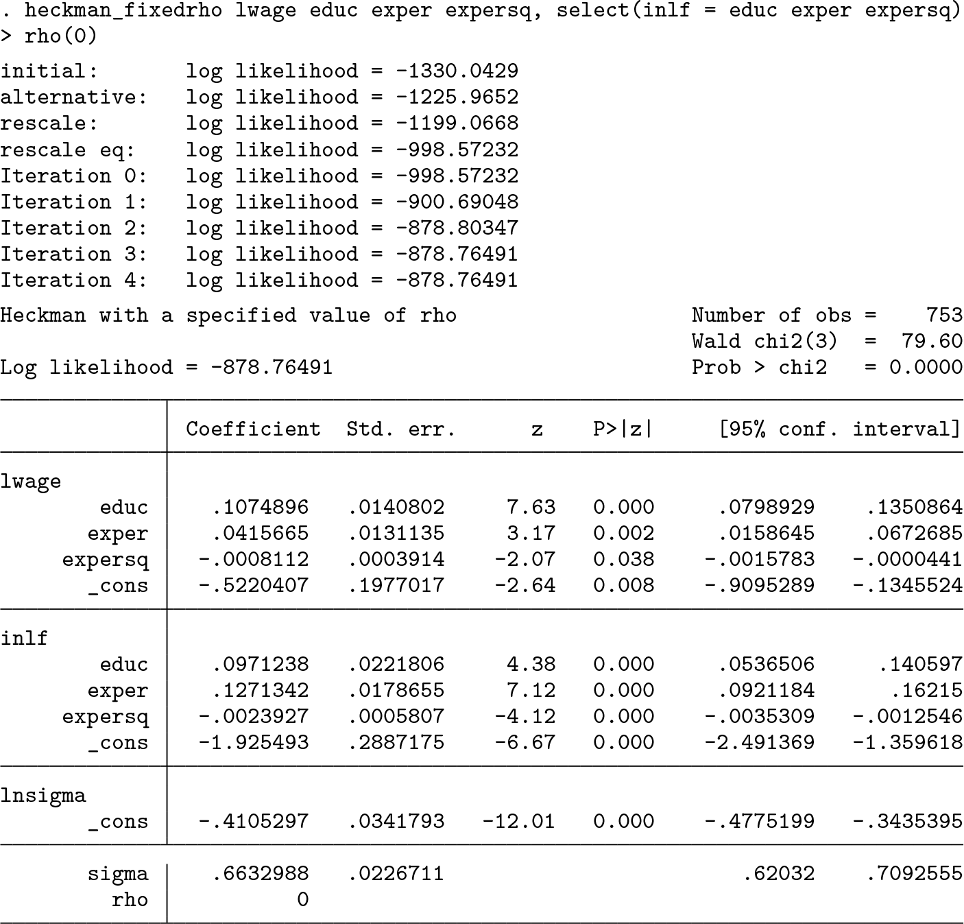
On the other extreme, we can see the results that would be found when fixing ρ at 0.99:

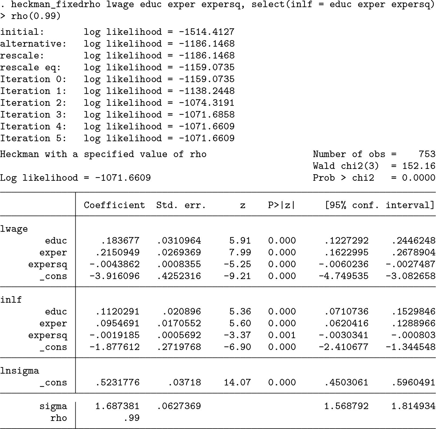
The coefficient on educ has increased from 0.107 to 0.184 because if the value of ρ was equal to 0.99, there would be a negative bias on educ when ρ is fixed at 0.

Seeing the possible values of the coefficient for different values of ρ provides bounds on the true value of the coefficient. In figure 2, we plot the estimated coefficient on educ as we vary ρ from 0 to 0.99.

Figure 2.

The estimated coefficient for various values of ρ

Finding maximum likelihood estimates

Our next example is a situation in which we have a valid exclusion and want to verify that we found the (true) maximum likelihood estimate. We use the specification from Zuehlke (2017), for which an author had reported a local rather than a global maximum of the likelihood function.

We begin with the Mroz dataset used in the previous example. We now use the data on family income (faminc) and the number of children (the sum of kidslt6 and kidsge6) for our excluded variables. Unlike the previous example, our dependent variable is now raw wage instead of log wage.

Set up by loading the dataset and creating two new variables:

Call heckman:

It is strange that Stata has reported a negative value of ρ; our intuition tells us that this should be positive.

Next we use heckman_scanrho, which will plot values of the likelihood function for each value of ρ:

The resulting plot is presented in figure 3. There is a root at ρ = −0.07, which is the result reported by Stata. The global maximum is around ρ = 0.89. Also note the difference in the log likelihoods reported for these two estimates. At the global maximum of 0.89, the log likelihood is −1, 518.58, whereas at −0.07 it is −1, 579.50.

Figure 3.

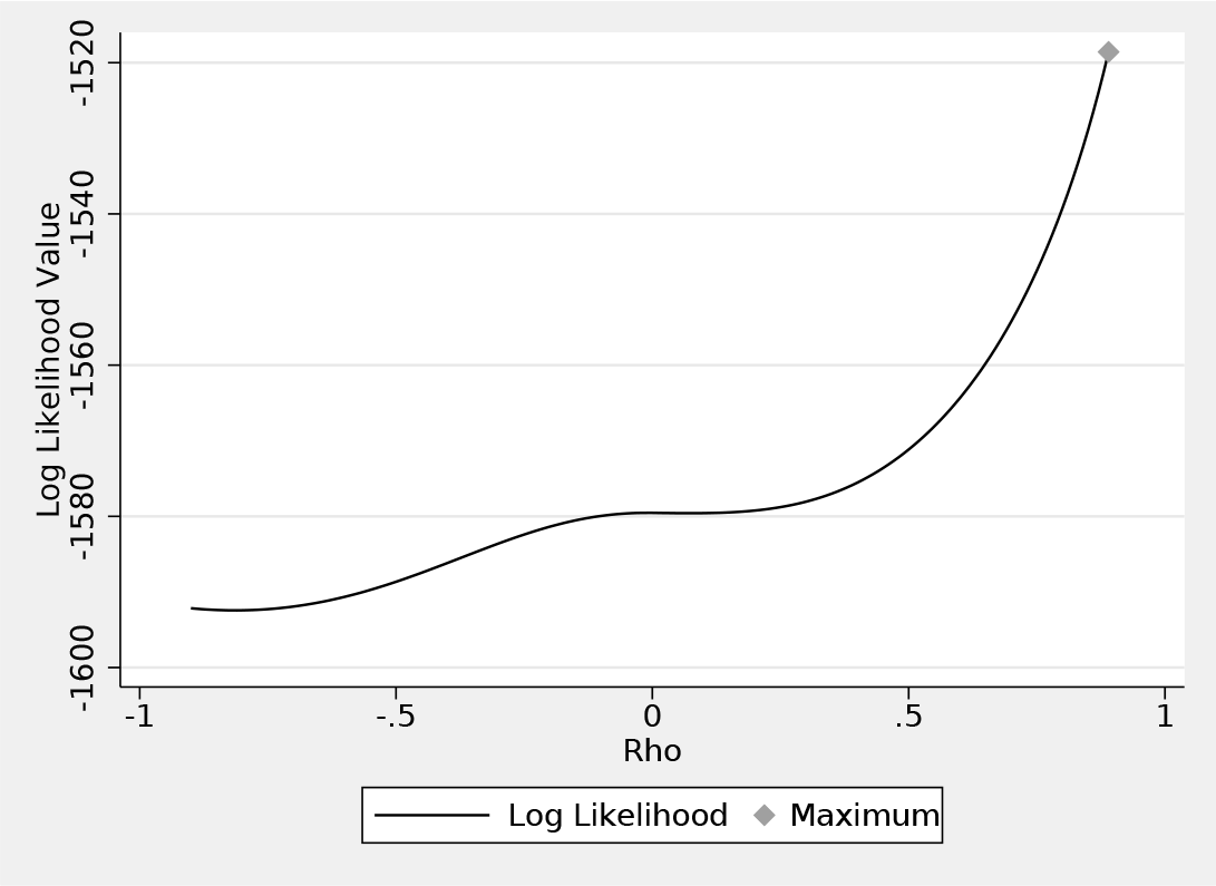
The value of the log-likelihood function for various values of ρ; the dot indicates the point at which the likelihood is maximized

By default, the step size is set to 0.01. It may be advisable to use a smaller step size to obtain a more accurate estimate. This may be especially helpful if the results of heckman_scanrho are being passed to heckman as initial values.

We can find the correct standard errors by setting initial values for Stata’s heckman command near the estimates found by heckman_scanrho. heckman_scanrho returns a matrix that can be passed to heckman as the initial values.

We first save this matrix: . matrix startv = e(init_values)

We then pass this matrix to heckman:

We are confident that these are the true maximum likelihood estimates from the plot in figure 3. Note that heckman_scanrho found that the value of ρ was 0.89 rather than 0.99 because, by default, heckman_scanrho will step through values of ρ equal to −0.90, −0.89,…, 0.89, and 0.90.

Comparing heckman estimates with those of heckman_fixedrho

Finally, we want to mention the differences between heckman and heckman_fixedrho when it is provided with the same value of ρ that was found by heckman. We use the specification from the previous example but return to using log wage instead of raw wage. First, we call heckman:

We now call heckman_fixedrho with the same value of ρ that was found by heckman:

The coefficients between these two are noticeably different. The source of difference is the maximization procedure being employed. The procedure used by heckman is preferable to the one used by heckman_fixedrho because it uses information about the first and second derivatives of the log-likelihood function. Notice that the log-likelihood value obtained by heckman is greater than the one obtained by heckman_fixedrho (−911.72 compared with −921.99). This is important: because heckman_scanrho calls heckman_fixedrho, the user needs to verify that the results found by heckman_scanrho do in fact improve the log likelihood relative to the results found by heckman.

5 Discussion and conclusion

Several extensions of this work are possible. We maintained the bivariate normality assumption in all of these models. This could be relaxed in several ways. Altonji, Elder, and Taber (2005) use Heckman and Singer’s (1984) approach for allowing for deviations for normality, which involves treating the stochastic terms as having a discrete component. Modeling the stochastic terms as a mixture of normals would also allow for some deviations from normality.

Another extension would be to change the maximization procedure used. Stata has several options for maximizing likelihood functions, which differ in whether derivatives of the likelihood functions are provided. The maximization methods that we used do not use any information about derivatives of the likelihood function. As a result, there may be specifications for which heckman converges but heckman_fixedrho does not converge (in addition to potential differences between the estimators as mentioned in the last example). This is because heckman uses information about the first and second derivative of the likelihood function.

The commands that we presented can be used to examine the sensitivity of regression results to sample selection or endogenous treatment and to verify that the results of a Heckman model are the global maximum of the likelihood function.

6 Programs and supplemental materials

Supplemental Material, sj-zip-1-stj-10.1177_1536867X211063149 - On identification and estimation of Heckman models

Supplemental Material, sj-zip-1-stj-10.1177_1536867X211063149 for On identification and estimation of Heckman models by Jonathan Cook, Joon-Suk Lee and Noah Newberger in The Stata Journal