Sage Journals: Discover world-class research

Abstract

Social scientists frequently rely on the cardinal comparability of test scores to assess achievement gaps between population subgroups and their evolution over time. This approach has been criticized because of the ordinal nature of test scores and the sensitivity of results to order-preserving transformations that are theoretically plausible. Bond and Lang (2013, Review of Economics and Statistics 95: 1468–1479) document the sensitivity of measured ability to scaling choices and develop a method to assess the robustness of changes in ability over time to scaling choices. In this article, I present the scale_transformation command, which expands the Bond and Lang (2013) method to more general cases and optimizes their algorithm to work with large datasets. The command assesses the robustness of an achievement gap between two subgroups to any arbitrary choice of scale by finding bounds for the original gap estimation. Additionally, it finds scale transformations that are very likely and unlikely to benchmark against the results obtained. Finally, it also allows the user to measure how much gap growth coefficients change when including controls in their specifications.

Keywords

st0652 scale_transformation test scores measurement achievement gaps robustness to scaling psychometrics

1 Introduction

With enrollments at a historical high for low- and middle-income countries, the focus in education has shifted away from enrollment and toward improving quality of education (World Bank 2018). Countries around the world are focusing on both increasing learning and closing substantial gaps across subpopulations, particularly in favor of disadvantaged groups. These gaps have been extensively documented in the United States, where much literature has identified stubborn test score gaps by sex (Bertrand and Pan 2013; Fryer and Levitt 2010), socioeconomic status (Reardon 2011, 2013), and race (Hanushek and Rivkin 2006; Clotfelter, Ladd, and Vigdor 2009; Fryer and Levitt 2004, 2006, 2013).

Gap measurement is essential to make inferences about equitable learning. What is surprising, though, despite the seemingly large gaps across subgroups, is that different studies often come to different conclusions. For instance, Fryer and Levitt (2004) first noted that a substantial black–white test score gap that had received extensive attention in the literature (see Coleman et al. [1966];¹ Kaufman and Kaufman [1983]; Krohn and Lamp [1989]; Phillips et al. [1998]; Phillips [2000]) disappeared after controlling for covariates. Additionally, they found that over the first four years of school, blacks lose about −0.10 standard deviations per year compared with other races. Bond and Lang (2013) then demonstrated that even this seemingly rock-solid racial gap in the United States is not robust to arbitrary scale transformations. That is, transformations that minimize or maximize learning by weighting test items differently, while still preserving order, create lower and upper bounds that are too wide to be informative or definitive.

These findings contribute to an ongoing debate around test score measurement, particularly on whether the assumptions that justify cardinality are satisfied in most tests (Ballou 2009; Ho 2009; Bond and Lang 2013; Jacob and Rothstein 2016). Three alternatives have been proposed. The first is to argue that the test at hand has been constructed in a manner that allows for cardinal measures of ability; this is the approach of the Rasch measurement, and Domingue (2014) provides statistical methods to verify the assumptions required for cardinality. The second is to give up on cardinality entirely and focus only on ordinal comparisons. Reardon et al.’s (2017) hetop command and Williams’s (2010) oglm command, as well as several official Stata commands, are designed to help users follow this approach.

A third approach, which this article focuses on, is to assess the robustness of findings to arbitrary scaling choices as proposed by Bond and Lang (2013). Specifically, their method builds on the idea that any monotone transformation of an ordinal scale is rank preserving and is therefore an equally valid measure of the underlying variable. They present an optimization method that searches for monotone transforms that minimize and maximize test score gaps, thus allowing researchers to provide bounds to their estimates of test score evolution across subgroups over time.² Here I extend their technique to more general cases and optimize their algorithm to work with large datasets. This allows for the simulation of multiple monotone transforms several times and bound differences by choosing transformations that maximize or minimize differences between subgroups.

2 Robustness to scaling

The ordinal nature of test scores implies that any monotonic transformation to a test score scale is potentially valid. We see this concept applied when colleges arbitrarily put more weight on grades from “harder” classes for admission purposes or when, within a particular test, a teacher decides that one question is worth more points because it is more “challenging”. Thus, when comparing test scores, we can ascertain only that someone with a high test score performed better than someone with a low one. It is much more difficult to know by how much. Standardizing test scores, which is the most common scale transformation, does not solve this issue. In fact, any analysis that relies on comparing standardized test scores implicitly assumes that test scores are interval scales. This assumption means that, in a scale from 0 to 100 points, the difference in underlying knowledge between individuals who scored 0 and 10 points is the same as that of those who score 90 and 100 points. In reality, this is seldom the case because there is no theoretical justification for this assumption; most exams have questions with varying levels of difficulty and use scales that are arbitrary in their mean, range, and distribution. Without interval scale properties, mean differences and standard deviations can be distorted depending on the weight each question receives.

Even when we equate test scores using item response theory, most of the time the underlying θ ability parameters obtained are ordinal in nature and defined only up to a linear transformation (see Lord [1975] and Ballou [2009] for a detailed explanation). Only in the very special case where all questions are equally informative (that is, the Rasch model) can item response theory scales be interpreted as interval scales. Nonetheless, this assumption is rarely fulfilled.

An assumption that is more reasonable and appropriate in most settings is that test scores are ordinal. Unlike temperature and distance, where the magnitude of a given difference corresponds to the same underlying measurement at different parts of the distribution, test score differences of the same “magnitude” can mean very different things at different points of the distribution. The only inference that we can make between someone with a score of 90 points and another person with a score of 100 is that the individual with a score of 100 demonstrated a larger amount of underlying knowledge or ability than the individual who scored 90.

Bond and Lang (2013) noted that the current literature does not adequately ensure that results are robust to scaling transformations and devised a methodology to find bounds for estimates measuring differences in test scores across subgroups and over time, such as the black–white test score gap in the United States. In particular, they created an algorithm that finds the upper and lower bounds for the estimates of differences in test scores across two subgroups at two points of time. To do so, they transform test scores using a sixth-degree polynomial monotonic transformation and optimize over the test score gap growth (that is, the difference in test scores between two subgroups in t ₀ minus the difference in t ₁) to make it as large or small as possible.

In the next section, I describe the step-by-step methodology developed by Bond and Lang (2013) and how the scale_transformation command extends their methodology for general use to a wide range of applications in this literature.

3 The scale_transformation command

3.1 Bond and Lang (2013) methodology

The Bond and Lang (2013) methodology tests the robustness to scaling of subgroup differences using arbitrary monotone transformations of an underlying ability or test score distribution. Relying on sixth-degree polynomial transformations, the original code tries to minimize or maximize the differences in test score growth between any two subgroups. These growth-minimizing and growth-maximizing transformations present lower and upper bounds, respectively, of the differences between subgroups.

Step-by-step methodology

1. Define the objective function as

Gap growth = α_{(1, t = 1)} - α_{(1, t = 0)}

where α _(1,t) is the difference in test scores between groups at time t (see step 2d for more details on how to obtain α _(1,t)). Note that test scores need to be already vertically equated. That is, they should be completely comparable and mapped into a single scale regardless of the time in which they were captured.

2. Optimize the following function over the defined objective:

Take the original test scores, and scale them down to be between 0 and 1 (for computational speed).

Transform original test scores (s) using a sixth-degree polynomial monotonic transformation T(s), optimizing over the gap growth by choosing five coefficients (β ₂ , β ₃ , β ₄ , β ₅, and β ₆) and one constant (c) for the polynomial transformation:

T (s) = β_{1} (s - c) + β_{2} {(s - c)}^{2} + β_{3} {(s - c)}^{3} + β_{4} {(s - c)}^{4} + β_{5} {(s - c)}^{5} + β_{6} {(s - c)}^{6}

Standardize transformed test scores in both periods (that is, t ₀ and t ₁) together. The original Bond and Lang (2013) code standardizes test scores separately, which could artificially increase or decrease the resulting gap. By jointly standardizing both years, we ensure that they remain vertically equated and that the resulting gap is only due to the transformations.

Run an ordinary least-squares regression separately for each period using a subgroup dummy and controlling for other desired variables. Given this setup, the coefficient on the subgroup dummy can be interpreted as the difference between each subgroup.

T {(s)}_{t} = α_{(0, t)} + α_{(1, t)} Group dummy + θ_{t} Controls

Find the gap growth between t ₀ and t ₁, as defined in step 1.

3. Run step 2 multiple times from different random starting values, checking that transformations preserve order (monotonic rule).

3.2 Improvements

The process described in section 3.1 is complex and computationally demanding. Most of the original public code is written in Mata, which might restrict its wider use among researchers. Furthermore, the public code was written for the specific estimation in their article. Thus, it makes some assumptions that might not necessarily extrapolate to other data and might affect the speed or magnitude of the results. This left space for two areas of improvement: 1) making the methodology more accessible to Stata users and 2) improving the precision, flexibility, and efficiency of the methodology.

In terms of accessibility, the scale_transformation command, together with this article and its documentation, will allow any Stata user to perform these robustness checks in one line of code.

Methodologically, the original process also sacrificed precision for efficiency. For instance, the parameter β ₁ was not optimized, and the monotonicity rule used did not check every single plausible value but rather checked monotonicity in small, equally spaced intervals. The scale_transformation command improves on these aspects as well as on computational speed.

Specifically, the original methodology has been improved by computing more accurate estimates (in quad precision) using QR decomposition tools in Mata. The monotonicity rule has also been enhanced to be more accurate and flexible with three variants: 1) a default rule that checks for monotonicity at every possible score value up to four decimals within the plausible range in a transformed scale between 0 and 1; 2) a quick rule that checks for monotonicity only at the unique score values present in the sample data; and 3) a theoretical rule that checks for monotonicity at every possible value using an external file. The last is of particular value if test scores come from a larger dataset that has scores for multiple years (that are not included in the optimization) or includes scores for subgroups not being analyzed. Furthermore, other options such as time-specific controls and weights have been included, as well as options to specify the number of times the command will run (yielding different results), the optimization methodology to be used at certain stages of the process, and the maximum number of iterations before the optimization cycle stops and returns results as if convergence were achieved.

Another important improvement of the scale_transformation command is that it is robust to transformations that fully change the sign of the gap regardless of its initial value. Because the optimization problem for the maximization or minimization gap growth options is complex and does not have a closed-form solution, in some specific cases, the maximization could yield the solutions for the minimization problem (and vice versa). The robust(integer) option allows the command to use the first K = integer iterations to check that the sign of the optimization is correct.

Finally, other robustness checks used by Bond and Lang (2013) have been added to the command. In particular, the scale_transformation command can search for transformations that maximize or minimize the correlation between initial and final test scores by looking at either the binary correlation between them or the resulting R-squared from regressing initial test scores on final test scores. These transformations allow the user to benchmark a likely or unlikely transformation and compare it with the results obtained when maximizing or minimizing the gap. Likewise, the command allows users to optimize over the absolute value of the difference between the gap growth calculated with and without controls. This additional check helps users to measure how much gap growth coefficients could change when including controls to their specifications.

3.3 Description

The scale_transformation command finds a monotonic transformation for a test score scale, which optimizes a specific objective function. The optimization object includes scores at two points of time for two comparison groups (for example, rich versus poor). This command performs a grid search from multiple random initial parameters to find the desired values. All the transformations found by this command are theoretically plausible given the ordinal nature of test scores.

A sixth-degree polynomial monotonic transformation is used because it provides flexibility to approach numerous continuous functions. Nevertheless, monotonicity checks need to be applied because this type of transformation does not necessarily preserve order. Furthermore, the monotonicity restriction introduces a discontinuity into the objective function that creates multiple local maximums and minimums. These characteristics yield a complex optimization problem that does not have a closed-form solution.

The scale_transformation command takes advantage of the Mata optimize() (see [M-5] optimize( )) function and performs a grid search to find multiple solutions. The results are reported in a dataset format that includes the values of the evaluated objective functions, the resulting parameters of each optimization iteration, and the initial parameters that yielded that result.

3.4 Syntax

scale_transformation, type( integer ) score1( varname ) score2( varname ) [compgroup( varname ) controls( varlist ) controls1( varlist )

controls2( varlist ) weights( varname ) iterations( integer ) maxoptiterations( integer ) singhmethod( integer ) bounddown( integer ) boundup( integer ) monotonicity( integer ) monofile( filename ) timeroff save( filename ) seed( integer ) robust( integer )]

3.5 Options

type(integer) indicates the type of optimization and the objective function to be performed. type() is required. integer is one of the following:

score1(varname) and score2(varname) specify, respectively, the variable that contains scores at (initial) period 1 and the variable that contains scores at (final) period 2. To improve processing speed, these variables are automatically scaled to be between 0 and 1 prior to running the command. The transformation used for this process is the same for the options score1() and score2() and does not affect the resulting estimations in any way. score1() and score2() are required.

compgroup(varname) specifies the variable that contains the group classification to be analyzed and from which the command will compare the top and bottom groups. This variable needs to be numeric. The command will take the lowest and highest values (that is, groups) and compare them while controlling for all other groups in the middle at the same time. Note that the option compgroup() should take on only integers greater or equal to 0 (all missings will be ignored). This option is allowed only when optimizing the gap growth or controls explanation (that is, type 1, 2, or 7).

controls(varlist) includes varlist as controls at both period 1 and 2. Variables should be numeric because they will be used directly in regressions. This option is allowed only when optimizing the gap growth or controls explanation (that is, type 1, 2, or 7).

controls1(varlist) includes varlist as controls at period 1 only. Variables should be numeric because they will be used directly in regressions. This option is allowed only when optimizing the gap growth or controls explanation (that is, type 1, 2, or 7).

controls2(varlist) includes varlist as controls at period 2 only. Variables should be numeric because they will be used directly in regressions. This option is allowed only when optimizing the gap growth or controls explanation (that is, type 1, 2, or 7).

weights(varname) uses varname as inverse probability weights. The default is weights(1).

iterations(integer) specifies the number of times the command will find optimal values using unique random-generated initial parameters. The default is iterations(1000). The more iterations there are, the longer the command will take to run and finish. Note that by default, if the command is stopped before ending, the results will not be stored. It is recommended that you test your command with a low number of iterations.

maxoptiterations(integer) specifies the maximum number of iterations before the optimization command stops and returns results as if convergence were achieved. The default is maxoptiterations(25), which in practice should be enough to achieve “convergence” with a fair degree of accuracy. This limit is necessary because the monotonicity restriction and complexity of the objective functions cause the optimization command to run indefinitely otherwise. See [M-5] optimize( ) for more details.

singhmethod(integer) specifies what the optimizer should do when, at an iteration step, it finds that H is singular. The default is singhmethod(1) for “hybrid” but can be changed to singhmethod(2) for “modified Marquardt algorithm”. See [M-5] optimize( ) for more details.

bounddown(integer) specifies the lower bound for the random-generated initial parameters for the optimization. This command creates random initial values and then uses them to find all the different local maximums or minimums accordingly. The default is bounddown(-1500).

boundup(integer) specifies the upper bound for the random-generated initial parameters for the optimization. This command creates random initial values and then uses them to find all the different local maximums or minimums accordingly. The default is boundup(1500).

monotonicity(integer) specifies the type of monotonicity check to be applied. The default is monotonicity(1) for “standard”, which checks for monotonicity at every possible score value (up to four decimals within the plausible range) in the original scale that was transformed to be between 0 and 1. When less precision is needed, monotonicity() can be set to 2 for “sample”, which checks for monotonicity only at the unique score values present in the sample data. If the test scores come from a larger dataset that has scores for multiple years, you can do a more thorough (but more time-consuming) check by putting together an external file with all theoretical or observed plausible scores where you want the command to check for monotonicity. For the latter, you must set monotonicity(3) for “external” and include the filename in monofile(filename). The plausible test scores in the “external” file should be in the original scale because the command will automatically transform them to the new scale and check for monotonicity at each of these transformed scores.

monofile(filename) specifies the file to be used when the monotonicity() type is set to 3 for “external”. This option should be used only with monotonicity(3). You can use .dta, .csv, .xls, or .xlsx files. Make sure that .csv, .xls, and .xlsx files have the name of the variable on the first row.

timeroff turns off the timer. The default is set to include the time (in minutes) that the command took to run, which is reported only if the command finishes.

save(filename) saves optimization results to filename once the command is done.

seed(integer) sets the seed for replication, where 0 <= integer <= 2147483647. If missing, the seed is randomly generated and included in the header of the command. Always save the log file to ensure you can recover the seed number for replication.

robust(integer) indicates the command to use the first K = integer iterations to check that the sign of the optimization is correct. Because the optimization problem for the maximization or minimization gap growth options (that is, type 1 or 2) is complex and does not have a closed solution, in some specific cases the maximization could yield the solutions for the minimization problem (and vice versa). To address this issue, you could activate the robust() option to use the first K = integer (where 20 <= K <= 300; K = even) iterations (in addition to N specified by the iterations() option) to check for a possible change of sign in max/min gap growth optimization results. Half the K iterations are used to find the maximization solution, while the other half of the K iterations are used for the minimization problem. Once the correct approach is selected, the command keeps the solutions for the correct specification and runs the remaining N iterations indicated in the iterations() option.

3.6 Optimization objectives

scale_transformation finds a sixth-degree polynomial monotonic transformation for a test score scale that optimizes one of the following:

Gap growth: gap difference between the bottom and top groups from the option compgroup() in period 2, minus the same gap difference in period 1. In other words, it is the difference between the regression coefficient of the top compgroup() indicator (controlling for groups in the middle) in period 2, minus the same regression coefficient of the top compgroup() indicator (also controlling for other groups in the middle) in period 1. In both, the coefficient of the top compgroup() indicator measures the difference between the top and bottom groups. Note that the gap growth is positive when the gap widens and negative when the gap shrinks (always with respect to the gap in period 1). Thus, the gap growth will always be negative when the coefficient changes signs between period 1 and 2 (regardless of whether it is from + to − or from − to +). Conversely, it will be positive when the gap widens, for instance, from −0.1 to −0.3.

Correlation: coefficient from regressing test scores in period 1 on test scores in period 2 (no controls allowed).

R-squared: from regressing test scores in period 1 on test scores in period 2 (no controls allowed).

Controls explanation: measures how much gap growth coefficients change when including controls in controls1(varlist) and controls2(varlist)—not in controls(varlist). This allows you to test the explanatory power of only a subset of desired control variables. That means that if you want to measure how much gap growth coefficients change by introducing time-invariant controls, you must include these variables in both controls1(varlist) and controls2(varlist). The controls explanation term is estimated by taking the distance (that is, absolute value of the difference) between the gap growth calculated without variables included in controls1() and controls2(), minus the gap growth calculated with these two controls’ varlists. To make the interpretation easier, both gap growths’ coefficients—with and without controls—are included in the results.

4 Resulting output

4.1 Example

In this section, we use timss_testscores.dta to find the gap growth maximization solution for test scores between year 1 and 2, comparing males and females:

Note that, given the above command, the command will run 40 times from different initial parameters and that each time, the command will report convergence after 15 iterations, performing a “sample” monotonicity check. Given the option robust(20), the command will use the first 20 simulations to check that the sign of the gap is correct by carrying out 10 maximizations and 10 minimizations. Once the correct direction is confirmed, the correct half is kept and the other discarded. Thus, in this example, the resulting dataset will contain only 30 observations.

Figure 1 shows the resulting dataset from the gap growth maximization example above. The missing values for the optimization object and transformation coefficients (that is, columns 1 through 8) correspond to transformations that are not order preserving. Thus, they are omitted in the final dataset.

Figure 1.

Resulting dataset from example

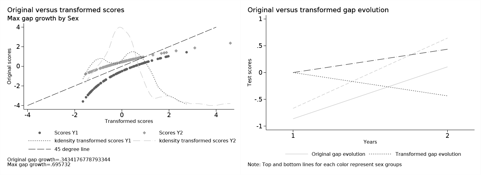
For this particular example, we can also plot the original and transformed scores to understand what the command did. Because we are searching for the gap growth maximization (that is, type(1)), we select the transformation that yields the highest gap growth from the resulting dataset, which is equal to 0.695732. Then, we use the corresponding coefficients and constant and apply the sixth-degree polynomial transformation in (1). Figure 2 plots the original versus transformed scores on the left and the test score gap evolution by sex between year 1 and 2. This particular gap growth maximization makes the gap in year 1 as small as possible while making the gap in year 2 as large as it can.

Figure 2.

Original versus transformed scores

Note that the original gap magnitude was 0.343418, about half the size of the transformed gap. These results are particular to this specific scenario, and in practice the algorithm might behave differently depending on the data and the objective function at hand.

4.2 Interpretation

Regardless of the optimization object chosen, the resulting dataset has a similar structure. Each row contains the results for one simulation. The obj variable contains the optimization object, while the rest of the variables contain the parameters of the sixth-degree polynomial transformation that achieves that object and the initial random starting values for these parameters. This format allows the user to not only have the full distribution of results but also access the necessary parameters to replicate the desired scale transformation if needed.

For the gap growth maximizing and minimizing options, one should be aware that the command finds the most extreme transformations, some of which might be extremely unlikely (although theoretically plausible). Thus, for instances where the bounds are too wide, it might be useful to benchmark against likely transformations (such as those found by the scale_transformation command that maximize correlation or R-squared) and explore other properties of test scores that could help us discard some of the most extreme and very unlikely transformations. For instance, Ho and Yu (2015) present values for skewness and kurtosis from 330 U.S. state-level examinations. Based on this, one could look at the moments of the resulting distributions and discard those that are extremely rare and unlikely to happen, thus narrowing the space between the resulting bounds.

5 Conclusion

One simple step that researchers can take to address some of the challenges of scaling and the ordinal nature of test scores is to test the robustness of their results to changes in the test score scales. The scale_transformation command allows anyone to implement several robustness checks to scaling decisions, particularly in the context of analyzing achievement gaps between subgroups in a panel setting. These checks build on the methodology developed by Bond and Lang (2013) and allow users to find bounds to the original gap estimation or transformations that are very likely or unlikely so as to benchmark against other results obtained. In practice, these are some of the essential checks that should be done when comparing test score averages over time and across subgroups.

When using the scale_transformation command, the researcher recognizes the ordinality of test scores and tests the robustness of his or her results to arbitrary monotonic transformations. This approach is more defensible theoretically and has the potential to discern real gaps from results that are significant only because of the arbitrary choice of scales made or taken as given.

Supplemental Material

Supplemental Material, sj-zip-1-stj-10.1177_1536867X211045574 - Test scores’ robustness to scaling: The scale_transformation command

Supplemental Material, sj-zip-1-stj-10.1177_1536867X211045574 for Test scores’ robustness to scaling: The scale_transformation command by Andres Yi Chang in The Stata Journal

Footnotes

6 Acknowledgments

I am grateful to Jishnu Das for his constant guidance, feedback, and encouragement to publish this article. I also thank Timothy Bond and Kevin Lang for their correspondence during the development of the article and command, as well as to Benjamin Daniels for his diligent feedback. Financial support for this research was made available through the World Bank Group Research Support Budget RSB714 grant. The findings, interpretations, and conclusions expressed in this article are those of the authors and do not necessarily represent the views of the World Bank, its executive directors, or the governments they represent.

7 Programs and supplemental materials

To install a snapshot of the corresponding software files as they existed at the time of publication of this article, type

Alternatively, install from the Statistical Software Components Archive:

. ssc install scale_transformation

You can also find the latest version of the program at

. net install scale_transformation,

> from(https://github.com/andresyichang/scale_transformation)

Notes

References

Ballou

2009. Test scaling and value-added measurement. Education Finance and Policy 4: 351–383. https://doi.org/10.1162/edfp.2009.4.4.351.

Bertrand

Pan

2013. The trouble with boys: Social influences and the gender gap in disruptive behavior. American Economic Journal: Applied Economics 5: 32–64. https://doi.org/10.1257/app.5.1.32.

Bond

T. N.

Lang

2013. The evolution of the black–white test score gap in grades K–3: The fragility of results. Review of Economics and Statistics 95: 1468–1479. https://doi.org/10.1162/REST_a_00370.

Clotfelter

C. T.

Ladd

H. F.

Vigdor

J. L.

2009. The academic achievement gap in grades 3 to 8. Review of Economics and Statistics 91: 398–419. https://doi.org/10.1162/rest.91.2.398.

Coleman

J. S.

Campbell

E. Q.

Hobson

C. J.

McPartland

Mood

A. M.

Weinfeld

F. D.

York

R. L.

1966. Equality of Educational Opportunity. Washington, DC: U.S. Government Printing Office.

Domingue

2014. Evaluating the equal-interval hypothesis with test score scales. Psychometrika 79: 1–19. https://doi.org/10.1007/s11336-013-9342-4.

Dorans

N. J.

Moses

T. P.

Eignor

D. R.

2010. Principles and practices of test score equating. ETS Research Report Series RR-10-29, Educational Testing Service. https://www.ets.org/Media/Research/pdf/RR-10-29.pdf.

Fryer

R. G.

Jr. Levitt

S. D.

2004. Understanding the black–white test score gap in the first two years of school. Review of Economics and Statistics 86: 447–464. https://doi.org/10.1162/003465304323031049.

Fryer

R. G.

Jr. Levitt

S. D.

2006. The black–white test score gap through third grade. American Law and Economics Review 8: 249–281. https://doi.org/10.1093/aler/ahl003.

10.

Fryer

R. G.

Jr. Levitt

S. D.

2010. An empirical analysis of the gender gap in mathematics. American Economic Journal: Applied Economics 2: 210–240. https://doi.org/10.1257/app.2.2.210.

11.

Fryer

R. G.

Jr. Levitt

S. D.

2013. Testing for racial differences in the mental ability of young children. American Economic Review 103: 981–1005. https://doi.org/10.1257/aer.103.2.981.

12.

Hanushek

E. A.

Rivkin

S. G.

2006. School quality and the black–white achievement gap. NBER Working Paper No. 12651, The National Bureau of Economic Research. https://doi.org/10.3386/w12651.

13.

A. D.

2009. A nonparametric framework for comparing trends and gaps across tests. Journal of Educational and Behavioral Statistics 34: 201–228. https://doi.org/10.3102/1076998609332755.

14.

A. D.

C. C.

2015. Descriptive statistics for modern test score distributions: Skewness, kurtosis, discreteness, and ceiling effects. Educational and Psychological Measurement 75: 365–388. https://doi.org/10.1177/0013164414548576.

15.

Jacob

Rothstein

2016. The measurement of student ability in modern assessment systems. Journal of Economic Perspectives 30: 85–108. https://doi.org/10.1257/jep.30.3.85.

16.

Kahlenberg

R. D.

2001. All Together Now: Creating Middle-Class Schools through Public School Choice. Washington, DC: Brookings Institution Press.

17.

Kaufman

A. S.

Kaufman

N. L.

1983. K-ABC: Kaufman Assessment Battery For Children: Interpretive Manual. Circle Pines, MN: American Guidance Service.

18.

Krohn

E. J.

Lamp

R. E.

1989. Concurrent validity of the Stanford–Binet fourth edition and K-ABC for head start children. Journal of School Psychology 27: 59–67. https://doi.org/10.1016/0022-4405(89)90031-9.

19.

Lord

F. M.

1975. Evaluation with artificial data of a procedure for estimating ability and item characteristic curve parameters. ETS Research Report Series 1975(2). https://doi.org/10.1002/j.2333-8504.1975.tb01073.x.

20.

Phillips

2000. Understanding ethnic differences in academic achievement: Empirical lessons from national data. In Analytic Issues in the Assessment of Student Achievement, ed. Grissmer

D. W.

Ross

J. M.

, 103–132. Washington, DC: U.S. Department of Education, National Center for Education Statistics.

21.

Phillips

Brooks-Gunn

Duncan

G. J.

Klebanov

Crane

1998. Family background, parenting practices, and the Black–White test score gap. In The Black– White Test Score Gap, ed. Jencks

Phillips

, 103–145. Washington, DC: Brookings Institution Press.

22.

Reardon

S. F.

2011. The widening academic achievement gap between the rich and the poor: New evidence and possible explanations. In Whither Opportunity? Rising Inequality, Schools, and Children’s Life Chances, ed. Duncan

G. J.

Murnane

R. J.

, 91–116. New York: Russell Sage Foundation.

23.

Reardon

S. F.

2013. The widening income achievement gap. Educational Leadership 70: 10–16.

24.

Reardon

S. F.

Shear

B. R.

Castellano

K. E.

A. D.

2017. Using heteroskedastic ordered probit models to recover moments of continuous test score distributions from coarsened data. Journal of Educational and Behavioral Statistics 42: 3–45. https://doi.org/10.3102/1076998616666279.

25.

Williams

2010. Fitting heterogeneous choice models with oglm. Stata Journal 10: 540–567. https://doi.org/10.1177/1536867X1101000402.

26.

World Bank. 2018. World Development Report 2018: Learning to Realize Education’s Promise. Washington, DC: The World Bank. https://doi.org/10.1596/978-1-4648-1096-1.

Supplementary Material

Please find the following supplemental material available below.

For Open Access articles published under a Creative Commons License, all supplemental material carries the same license as the article it is associated with.

For non-Open Access articles published, all supplemental material carries a non-exclusive license, and permission requests for re-use of supplemental material or any part of supplemental material shall be sent directly to the copyright owner as specified in the copyright notice associated with the article.

0.03 MB

0.00 MB