icio: Economic analysis with intercountry input–output tables

Abstract

Several new statistical tools and analytical frameworks have been recently developed to measure countries’ and sectors’ involvement in global value chains. Such a wealth of methodologies reflects the fact that different empirical questions call for distinct accounting methods and different levels of aggregation of trade flows. In this article, we describe icio, a new command for the computation of the most appropriate measures of trade in value added as well as participation in global value chains. icio follows the conceptual framework proposed by Borin and Mancini (2019, Policy Research Working Paper WPS 8804; WDR 2020 Background Paper, World Bank Group), which in turn extends, refines, and reconciles the other main contributions in this strand of the literature. icio is flexible enough to work with any intercountry input–output table and with any level of aggregation of trade flows.

1 Introduction

The diffusion of global production networks has called for new statistical tools providing a representation of complex production linkages between and within economies. New types of data sources, the intercountry input–output (ICIO) tables, and new analytical frameworks have been developed to measure supply-and-demand contributions of countries and sectors in global value chains (GVCs). ¹ In a nutshell, these frameworks decompose gross exports in terms of their value-added components. This is crucial to unravel production–demand linkages at the global level because, in a world of GVCs, exports embed a relevant amount of imported intermediate inputs. In addition, the direct importer often differs from the market of final absorption. Thus, nowadays traditional trade statistics alone cannot provide an adequate representation of supply and demand interlinkages.

In this article, we describe icio, a new command for the computation of countries’ and sectors’ participation in GVCs. The command follows the conceptual framework proposed by Borin and Mancini (2019), which in turn extends, refines, and reconciles the other main contributions in this strand of the literature. icio also computes the most relevant measures of trade in value added.

icio is flexible in many aspects. It allows the user to choose from different accounting methodologies, called “perspectives”. Each of these perspectives is best suited to address specific empirical questions, such as tracking production–demand linkages, assessing countries’ participation in global production sharing, quantifying value added embedded in countries’ and sectors’ exports, and evaluating the potential exposure to macroeconomic and trade policy shocks. It exploits the most famous ICIO tables—the World Input–Output Database (WIOD) (Timmer et al. 2015), the Organisation for Economic Co-operation and Development (OECD) Trade in Value-Added (TiVA) Database (OECD 2018), the Eora Global Supply Chain Database (Lenzen et al. 2013), and the Asian Development Bank (ADB) Multiregional Input–Output Table (MRIOT) Database. ² Moreover, it is straightforward to load and use any user-provided ICIO table to compute value-added trade and GVC participation measures.

More specifically, icio encompasses the most relevant measures of value added in exports and imports at the aggregate, bilateral, and sectoral levels. For a given trade flow, it disentangles the source country and sector and the destination country and sector of value-added content. Moreover, for export flows at any level of disaggregation, icio computes the component related to GVCs trade, that is, the one entailing more than a single border crossing. This measure—and its backward and forward GVCs participation subcomponents—is featured in the World Bank’s World Development Report (WDR) 2020 (World Bank 2019). ³

In addition, the icio command can be used to retrieve, from the ICIO tables, the gross domestic product (GDP) (that is, value added) produced by a given country or industry (origin), the final demand in different countries and sectors (destination), or a combination of the two (when both origin and destination are specified).

We believe that the icio command can provide a fully exhaustive representation of supply–demand linkages between countries and sectors through an accurate decomposition of gross trade flows. In this way, the command can address a broad set of empirical questions, summarized in table 2. We plan to build new commands that share with icio the same structure and exploit the same data sources but focus on other specific aspects. ⁴

The rest of the article is organized as follows. In section 2, we show how to load ICIO tables by using the icio_load command. In section 3, we show how supply, demand, and supply–demand linkages can be computed exploiting icio. This is useful when the empirical questions are related to supply or demand or require linking the origin of the value added to its absorption in final demand, without considering explicitly international trade flows. In section 4, we provide the tools to obtain value-added decompositions of trade flows by country of origin and destination. In section 5, we focus on the measurement of GVC participation. In several instances and for illustration, we show how to replicate some of the measures of GVC participation and figures presented in the World Bank’s WDR 2020. Section 6 concludes.

Each section shares the same structure. At the beginning, we provide a brief overview of the measures therein discussed. Then, we present the related conceptual framework and discuss, through examples, the relevant icio syntax.

2 ICIO tables

Input–output (IO) models were developed by Leontief (1936) to represent and analyze production and consumption relationships within an economy. The related statistical tools, the IO tables, report the monetary amount of inputs of each sector necessary to produce the total output of a given industry and, in turn, show how this output is used as final consumption (or investment) or as intermediate inputs for other productions. National IO tables distinguish only between domestic and foreign inputs; on the output side, exports represent one of the possible “final” uses of output, as domestic consumption and investment. ICIO tables, which have been developed combining national IO statistics with trade data, describe sale–purchase relationships between industries within and between economies as well as the uses in different final-demand components (for example, consumption, investment, and government spending). In particular, an ICIO table specifies the country–sector pairs that provide intermediate inputs to a given industry and the country–sector pairs to which that industry sells its output—in the case of intermediate products—or the ultimate destination markets for final goods.

In section 2.1, we present the basic conceptual framework of ICIO models, while in section 2.2, we show how to load ICIO tables with the icio_load command.

2.1 Conceptual framework: ICIO models

A generic ICIO model with G countries and N sectors can be represented by the scheme in figure 1, where Z _ij is the N×N matrix of intermediate inputs produced in country i (rows) and used in country j (columns), Y _ij is the N × 1 vector of final goods and services completed in country i and absorbed in country j, X _i is the N ×1 vector of gross output produced in country i, and VA _i is the 1 × N vector of value added generated in country i.

Figure 1.

ICIO scheme

The specific column j, n of the ICIO table in figure 1 shows how the output of country j and sector n (x_j,n ) is produced: sourcing intermediate inputs from the same and other country–sector pairs and adding its own value added, $\left(x_{j,n}={\displaystyle {\sum }_i^G{\displaystyle {\sum }_m^N{z}_{ij,mn}}}+v{a}_{j,n}\right)$ . In turn, the row j, n shows how the output of country j and sector n is used: that is, as intermediate inputs for different industries and countries and as final products to serve domestic and foreign, demand $\left(x_{j,n}={\displaystyle {\sum }_i^G{\displaystyle {\sum }_m^N{z}_{ij,mn}}}+{\displaystyle {\sum }_i^G{y}_{ji,n}}\right)$ . IO models hinge upon key proportionality assumptions: the input composition in sectoral productions does not change by geographical destination of output, and it is identical between intermediate and final goods.

2.2 Implementation: Loading ICIO tables using the icio_load command

To use the icio command, one needs to load a particular ICIO table by using the icio_load command. icio_load allows the user to work directly with the most popular ICIO tables—the OECD TiVA Database (OECD 2018), WIOD (Timmer et al. 2015), the Eora Global Supply Chain Database (Lenzen et al. 2013), and the ADB MRIOT Database. In addition, any other user-provided ICIO table can be loaded.

2.2.1 Syntax

The basic syntax for icio_load is

icio_load,[ icio_load_options ]

For the full list of options, see help icio. The main options are as follows:

iciotable( table_name [ , usertable_options ] ) specifies the ICIO table to be used for the analysis. The default is wiodn, the last WIOD release available (release 2016; see below for more details on the available tables’ versions). See help icio for details on the table_name and usertable_options options.

year( #) sets the year to be used for the analysis. The default is the last available year: year(2014) for the WIOD tables (wiodn), year(2015) for TiVA tables (tivan), year(2015) for the Eora Global Supply Chain Database tables (eora), and year(2019) for the ADB MRIOT Database (adb). This option is not needed for user-provided tables.

info shows the data sources and the versions of the loadable ICIO tables.

2.2.2 Examples

icio_load can be used for the following purposes:

• 1. To display the list of the directly available ICIO tables and their releases: ⁵

  

  In this way, the user can always recover which ICIO tables are directly available via the icio command. As can be seen from the previous output, at the time of writing, the following tables have been made available: the 2013 and the 2016 releases of the WIOD tables, the 2016 and 2018 releases of the TiVA tables, the 199.82 version of the Eora Global Supply Chain Database tables, and the 2021 release of the ADB MRIOT Database.

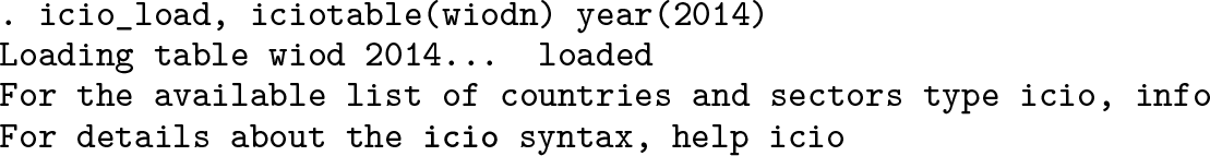
• 2. To load a specific year of the ICIO table of interest. For example, the following syntax allows the user to load the year 2014 of the WIOD tables released in 2016 (that is, wiodn): ⁶

  

• 3. To load a user-provided ICIO table by specifying user instead of a specific ICIO table’s code in the iciotable( table_name [ , usertable_options ] ) option. The user-provided ICIO table and the related country list must be provided using two different comma-separated files (that is, files with extension .csv). For example,

  

  The syntax above shows that the following additional information has to be provided for loading a user-provided table: i) the path to the folder where the .csv file containing the table is located, via the suboption userpath( string); ii) the name of the .csv file containing the table, via the suboption tablename( string); and iii) the name of the file containing the country list, via the suboption countrylistname( string).

  Notice that the table’s .csv file must contain only one matrix of dimension (G × N) × (G × N + G × U), where G is the number of countries, N is the number of sectors, and U is the number of uses (that is, consumption, investment, etc.). See help icio for more details.

3 Supply, demand, and supply–demand linkages

ICIO tables can be used in combination with long-established accounting relationships (Leontief 1936) to measure the net value of production (GDP) of a country or sector and the value of final demand in a given country or sector, and to pin down the links between the country or sector where the value added originates and the market where it is absorbed in final demand.

In section 3.1, we show how to retrieve from ICIO tables supply, demand, and supply– demand linkages—that is, GDP by country or sector of origin, destination, or both— while in section 3.2, we provide some examples to illustrate how these measures can be computed using icio.

3.1 Conceptual framework: Supply and demand in ICIO models

Given a country s, each unit of its gross output can be either consumed as a final good or used as an intermediate good at home or abroad:

$X_s={\displaystyle \sum _r^G\left(A_{sr}{X}_r+Y_{sr}\right)}$

1

Country r can be either s itself or any given importing country, and A is the GN×GN matrix of intermediate input coefficients, obtained by dividing Z by X [that is, A = Z ø (u ⊗ X ′)], where u is a 1 × GN vector of ones.

Then the basic relationship between gross output and final demand is given by

$X={(I-A)}^{-1}Y=BY$

2

where B is the GN×GN “global” Leontief inverse that measures the total units of gross output in countries and sectors of origin necessary to produce a certain unit of final goods and services. Indeed, B accounts for all the gross output produced in all the rounds of production because B = I + A + A ² + A ³ + · · · + A ⁿ = (I − A) ^{− 1}.

In each production stage, some value added is generated. The value-added share in each unit of gross output produced by country s (V _s ) is equal to 1 minus the sum of the direct intermediate input shares of all the domestic and foreign suppliers (that is, $V_s=u_N\left[I-{\displaystyle {\sum }_r^G{A}_{rs}}\right]$ ), where u _N is a 1 × N vector of ones. Then the direct domestic value-added matrix for all countries can be defined as

$V=\left[\begin{array}{cccc}{V}_1& 0& \cdots & 0\\ 0& V_2& \cdots & 0\\ ⋮& ⋮& \ddots & ⋮\\ 0& 0& \cdots & V_G\end{array}\right]$

Premultiplying the right-hand side of (2) by V, it is possible to obtain a G×G GDP matrix reporting the GDP by country pairs of source (rows) and absorption (columns).

$GDP=\left[\begin{array}{cccc}{V}_1{\displaystyle {\sum }_r^G{B}_{1r}{Y}_{r1}}& V_1{\displaystyle {\sum }_r^G{B}_{1r}{Y}_{r2}}& \cdots & V_1{\displaystyle {\sum }_r^G{B}_{1r}{Y}_{rG}}\\ V_2{\displaystyle {\sum }_r^G{B}_{2r}{Y}_{r1}}& V_2{\displaystyle {\sum }_r^G{B}_{2r}{Y}_{r2}}& \cdots & V_2{\displaystyle {\sum }_r^G{B}_{2r}{Y}_{rG}}\\ ⋮& ⋮& \ddots & ⋮\\ V_G{\displaystyle {\sum }_r^G{B}_{Gr}{Y}_{r1}}& V_G{\displaystyle {\sum }_r^G{B}_{Gr}{Y}_{r2}}& \cdots & V_G{\displaystyle {\sum }_r^G{B}_{Gr}{Y}_{rG}}\end{array}\right]$

More specifically, the GDP produced in country s can be computed as

$GD{P}_s=V_s{\displaystyle \sum _k^G{\displaystyle \sum _l^G{B}_{sk}}}{Y}_{kl}=\underset{\begin{array}{c}\text{ domestically }\\ \text{ absorbed GDP }\end{array}}{\underbrace{V_s{\displaystyle \sum _k^G{B}_{sk}}{Y}_{ks}}}+\underset{\begin{array}{c}\text{ GDP absorbed }\\ \text{ abroad }\left(VA{X}_s\right)\end{array}}{\underbrace{V_s{\displaystyle \sum _k^G{\displaystyle \sum _{l\ne s}^G{B}_{sk}}}{Y}_{kl}}}$

3

where we have singled out the part that is absorbed at home and the part that is finally consumed abroad in country l, as a final good assembled in country k, which correspond to the “value-added exports” as defined by Johnson and Noguera (2012).

It is also possible to decompose the final demand (FD) of country s by distinguishing between the part of value added domestically produced and the part that originates abroad:

$F{D}_s={\displaystyle \sum _j^G{\displaystyle \sum _k^G{V}_j}}{B}_{jk}{Y}_{ks}=\underset{\begin{array}{c}\text{ domestically }\\ \text{ produced FD }\end{array}}{\underbrace{V_s{\displaystyle \sum _k^G{B}_{sk}}{Y}_{ks}}}+\underset{\begin{array}{c}\text{ FD produced }\\ \text{ abroad }\end{array}}{\underbrace{{\displaystyle \sum _{t\ne s}^G{V}_t}{\displaystyle \sum _k^G{B}_{tk}}{Y}_{ks}}}$

4

To get a decomposition of GDP by sectors of origin, it is sufficient to substitute the direct value-added V _s in (3) and (4) with its diagonalized form ${\widehat{V}}_j$ (that is, the N×N diagonal matrix with the direct value-added coefficients along the principal diagonal and 0s elsewhere). Similarly, the decomposition by sectors of final absorption is obtained by replacing the vector of final demand with its diagonalized form. For instance, for goods completed in country k and absorbed in country l, the N×N diagonal matrix of final demand is

${\widehat{Y}}_{kl}\equiv \left[\begin{array}{cccc}{y}_{kl,1}& 0& \cdots & 0\\ 0& y_{kl,2}& \cdots & 0\\ ⋮& ⋮& \ddots & ⋮\\ 0& 0& \cdots & y_{kl,N}\end{array}\right]$

Then the decomposition of value added by combinations of country or sector of origin and country or sector of final destination can be obtained from the GN×GN matrix

$\mathbf{\text{VA}}(\text{origin/destination})=\widehat{V}B\widehat{Y}$

5

3.2 Implementation: Supply and demand with icio

The icio command can be used (i) to retrieve the GDP (that is, value added) produced by a given country or industry (origin of value added) by specifying the option origin(), (ii) to measure the final demand in different countries and sectors (destination of the value added) by specifying the option destination(), or (iii) to find a combination of the two (both origin() and destination()).

3.2.1 Syntax

1. Gross domestic product (GDP):

icio, origin(country_code [ , sector_code ] ) [ standard_options ]

2. Final demand:

icio, destination(country_code [ , sector_code ] ) [ standard_options ]

3. Value added by origin and final destination:

icio, origin(country_code [ , sector_code ] ) destination(country_code [ , sector_code ] ) [ standard_options ]

The list of available country–sector codes for the loaded ICIO table can be displayed by running icio, info. The standard_options are as follows:

save(filename [ , save_options ] ) saves the icio output (scalar, vector, or matrix) to an Excel file (with the .xlsx extension).

groups( grouping_rule group_name [,… ] ) specifies a user-defined grouping of countries. In this way, output measures can be computed for a country group (for example, the “Euro area”, “MERCOSUR”, or “ASEAN”) as a whole while accounting for the specific supply/demand/trade structure of each member of the group. To define one or more country groups, the user has to provide a list of comma-separated country codes, which is the grouping_rule, followed by a user-defined group_name.

As for the save_options of save(), the user can specify replace to overwrite an existing Excel file, modify to modify an existing Excel file, and sheet(sheetname [, replace ] ) to specify the worksheet to use. The default sheetname is icio_out. These three options mimic exactly those of the putexcel set command (see help putexcel).

3.2.2 Stored results

icio stores the following in r():

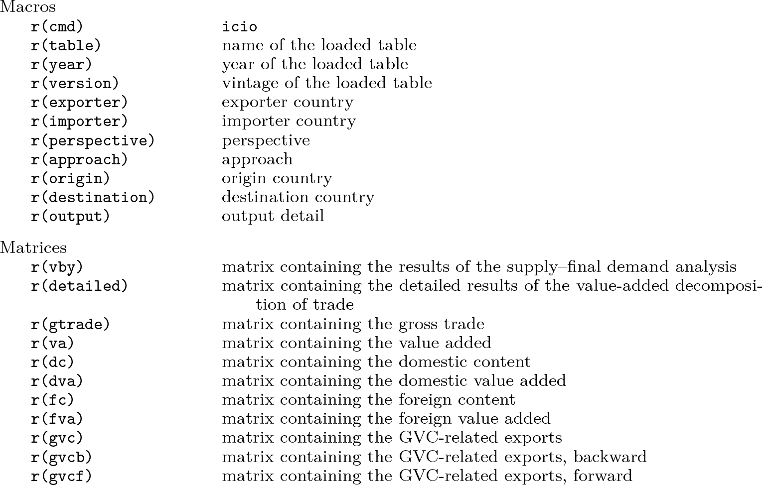
3.2.3 Examples

icio is useful to address empirical questions related to supply, demand, and supply– demand relationships without considering explicitly international trade flows. For instance, it is possible to retrieve the GDP of Germany that is finally absorbed in China (that is, “value-added exports” [Johnson and Noguera 2012]), that according to the WIOD database in 2014 is

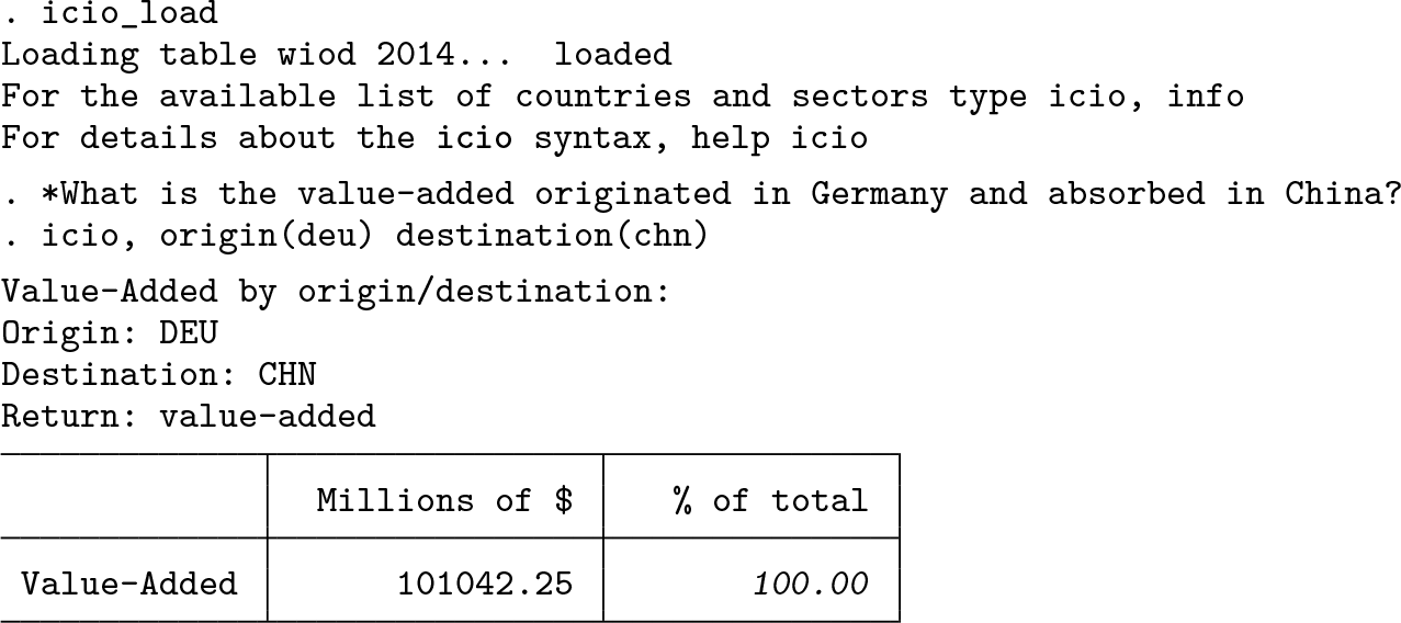
The Stata output displays the value in millions of U.S. dollars and the share of total value added produced in a specific country, when the complete list of countries or sectors of destination is selected by specifying the code all ⁷ (or absorbed by a specific country or sector, if the complete list of countries or sectors of origin is specified with the same code). ⁸ If the option all is not specified, the share will be clearly equal to 100%. For example,

As can be noted, the share of the German GDP absorbed in China (on the total GDP produced by Germany), which is around 2.8%, is obtained either by looking for the CHN row in the previous output or by taking the ratio of the dollar values obtained through the options origin(deu) and destination(chn) and the value of the total German GDP, which can be obtained using

Other examples of questions that could be answered (see the reported syntax) with the analysis of supply–demand linkages through icio are

• What is the GDP (value added) produced by each country?

icio, origin(all)

• How much value added does each country produce in a given sector (for example, sector code 19)?

icio, origin(all, 19)

• What is the aggregate final demand of each country?

icio, destination(all)

• Where is the value added produced in the Italian sector 19 absorbed?

icio, origin(ita, 19) destination(all)

• Which final demand sectors in China are the most important for the absorption of U.S.-made value added?

icio, origin(usa) destination(chn, all)

• Where is the GDP produced in each country absorbed (and save the output as “supply_demand” Excel file in the current working directory)?

icio, origin(all) destination(all) save(supply_demand)

• How much is the U.S.–Mexico–Canada Agreement (formerly North American Free

Trade Agreement) countries’ final demand in sector 20 satisfied by Chinese productions?

icio, origin(chn) destination(usmca,20) /// groups(usa, mex, can, "usmca")

4 Value added in trade flows

The accounting relationships presented in the previous section provide a useful tool to link the origin of value added (GDP) to its absorption in final demand. However, they provide only partial information on overall production processes and cross-country relationships. For instance, no information is provided on the production stages that take place nor on the national borders that are crossed between the stage in which the value added is generated and the stage of its final absorption. Both of the above represent critical information to understand countries’ interdependence in GVCs.

In many empirical applications, it is important to trace value added in gross trade flows, for instance, when we want to measure the value added produced by a country that is involved in a certain trade relationship. Depending on the empirical issue under investigation, it is also necessary to consider trade flows at different levels of disaggregation and analyze their value-added content. In fact, in some cases, we may be interested just to single out the value added embedded in global trade flows or in the total exports or imports of a country. In other cases, the bilateral and sectoral dimensions of trade flows may also matter. For instance, when studying the implications of GVCs, it is relevant to consider the position of a country (or sector) within the production chain and identify its direct upstream and downstream trade partners. This may be relevant to geographically map the production networks and analyze the international propagation of macroeconomic shocks.

A key issue in the value-added accounting of trade regards the definition of “doublecounted” components, that is, items that are recorded several times in a given gross trade flow because of the back-and-forth shipments that occur in a cross-national production process (Koopman, Wang, and Wei 2014). For instance, imagine that a country is exporting cotton. After some processing stage abroad, the cotton is imported back, embedded in some fabric, to be further reexported as apparel. The value of cotton will be counted twice in the aggregate exports of the country, that is, “double counted”—in the first export flow and in the second one, embedded in the apparel—but once in the GDP (that is, value added).

Now imagine that the goal is to allocate the value added across the two export flows. A reasonable way is to consider the cotton production as value added in the first shipment of cotton, and as double counting in the second one, when cotton is embedded in the shipment of apparel. Summing the value-added terms in the two export flows, we end up with consistent aggregate figures at the country level, that is, cotton classified once as value added and once as double counting.

Consider now a different goal, that is, assessing the value added exposed to a specific trade barrier imposed by a partner. To this end, suppose that a tariff impairs the exports of apparel. Now when considering the value added embedded in the second flow, the one exposed to the tariff, that flow of cotton also needs to be accounted for. In this way, we are able to correctly assess the value added that could be impaired by the tariff.

More in general, depending on the type of trade flow and the objective of the analysis, it is necessary to define the “perimeter” according to which something is classified as value added or double counted, that is, a specific accounting “perspective” has to be chosen.

Each perspective is better suited to address specific empirical issues. Whenever the empirical application requires to retrieve the entire value added of a country or sector of origin that is embedded in a given trade flow, as in the second example above, the accounting perspective to be chosen should match the level of disaggregation of the trade flow considered, as reported in the first column of table 1 (for example, “exportingcountry” perspective for aggregate exports, “bilateral” perspective for an aggregate bilateral trade flow, “sectoral-bilateral” perspective for a trade flow between two countries in a given sector, etc.). ⁹ For instance, suppose a tariff is imposed on the imports of a given sector from a certain partner, and we are interested in evaluating what part of the exporting-country GDP is exposed to the tariff. In this case, we want to consider as value added the entire GDP that is involved in this sectoral-bilateral relationship, even if part of that was previously exported to other countries or sectors (that is, double counted in an exporting-country perspective). The specific sectoral-bilateral relationship becomes the new relevant perimeter, and only the items that enter multiple times in this trade flow are considered as double counted. Indeed, this is what is called a sectoral-bilateral perspective, the one used in the second example on cotton.

Table 1.

A summary of the available perspectives and approaches for each trade flow

	Perspective in line with the trade flow (1)	Perspective consistent with more aggregate flows (that is, additive) (2)
1. Total exports 1a. Aggregate 1b. Sectoral	Exporting country Sectoral-exporter	World (source/sink) Exporting country (source/sink)
2. Bilateral exports 2a. Aggregate 2b. Sectoral	Bilateral Sectoral-bilateral	Exporting country (source/sink) Exporting country (source/sink)
3. Total imports 3a. Aggregate 3b. Sectoral	Importing country Sectoral-importer	not applicable not applicable

However, these measures cannot be summed up to get a precise assessment of valueadded contents in more aggregate trade flows, for example, value added in the total exports of a country. In other words, they are nonadditive. ¹⁰ Thus, if we are looking for a breakdown of the value-added measures by sectors of exports, by importing partners, or by sector–partner combinations, consistent with exporters’ aggregate figures as in the first example on cotton, we need to apply the exporting-country perspective also to the decomposition of more disaggregated trade flows (see column two of table 1). In this way, the resulting measures are additive; that is, measures at a more aggregate level can be obtained by summing disaggregate results. This accounting perspective also can be used for other purposes, such as, for instance, to single out the portion of trade in any type of export that crosses just one international border. Indeed, section 5 shows that this is instrumental for measuring GVC-related trade.

Whenever the perspective is set at a more aggregate level compared with the considered trade flow, it is also needed to select an approach to allocate double counting. icio implements two alternative approaches: ¹¹ the first method, the so-called “source-based” approach, accounts for the value added the first time it leaves the country of origin; the second, “sink-based” approach considers it the last time it crosses the national borders. The choice between these two approaches depends on the particular issue we want to address. The source approach is designed to examine the production linkages and the country (and sector) participation to different types of production processes. This makes it more suited to assess, for instance, the share of an export flow that crosses just one border (traditional exports) as opposed to the share that is further reexported (GVC exports). Conversely, the value added in the sink approach is recorded as closely as possible to the moment when it is ultimately absorbed. This makes it more suited to studying the relationship between value added in exports and final demand, as in the analysis of bilateral trade balances.

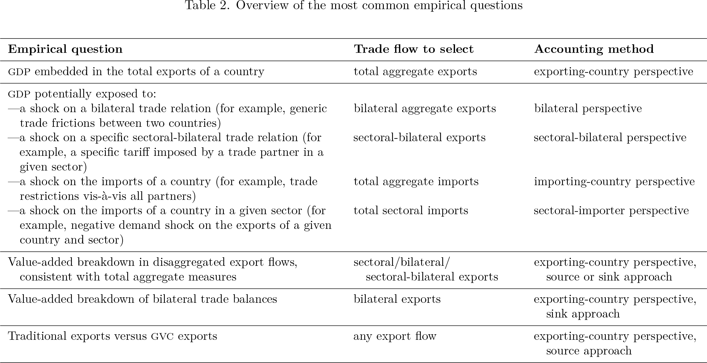
As already mentioned, each perspective is suited to address specific empirical questions. In table 2, we provide a nonexhaustive overview of the most common ones, along with the best-suited accounting method to provide an answer. See section 4.4 for additional examples together with the related icio syntax.

Table 2.

Overview of the most common empirical questions

Empirical question	Trade flow to select	Accounting method
GDP embedded in the total exports of country	total aggregate exports	exporting-country perspective
GDP potentially exposed to: —shock on bilateral trade relation (for example, generic trade frictions between two countries) —shock on specific sectoral-bilateral trade relation (for example, specific tariff imposed by trade partner in given sector) —shock on the imports of country (for example, trade restrictions vis-à-vis all partners) —shock on the imports of country in given sector (for example, negative demand shock on the exports of given country and sector)	bilateral aggregate exports sectoral-bilateral exports total aggregate imports total sectoral imports	bilateral perspective sectoral-bilateral perspective importing-country perspective sectoral-importer perspective
Value-added breakdown in disaggregated export flows, consistent with total aggregate measures	sectoral/bilateral/sectoral-bilateral exports	exporting-country perspective, source or sink approach
Value-added breakdown of bilateral trade balances	bilateral exports	exporting-country perspective, sink approach
Traditional exports versus GVC exports	any export flow	exporting-country perspective, source approach

In the next sections, we show the conceptual framework of the value-added accounting in total exports, following an exporting-country perspective (section 4.1), in bilateral exports, both with a bilateral and an exporting-country perspective (section 4.2), and in all the possible trade flows (section 4.3). Then in section 4.4, we show the implementation in icio and provide some empirical examples with the related syntax.

4.1 Conceptual framework: Value added in total exports

The problem of isolating value added in trade flows has been addressed at length in the literature. ¹² To provide a useful starting point, we begin from the analysis of the aggregate exports of a country. Gross exports of country s can be broken down according to the country that initially produced each component. The part that originated in country s itself is referred to as the “domestic content of exports” (DC _s ), whereas the remaining part is called the “foreign content of exports” (FC _s ; Koopman et al. [2010])

$u_N{E}_{s*}=\underset{\begin{array}{c}\text{ domestic }\\ \text{ content }\left(D{C}_s\right)\end{array}}{\underbrace{V_s{B}_{ss}{E}_{s*}}}+\underset{\begin{array}{c}\text{ foreign }\\ \text{ content }\left(F{C}_s\right)\end{array}}{\underbrace{{\displaystyle \sum _{t\ne s}^G{V}_t}{B}_{ts}{E}_{s*}}}$

6

Although the above formula closely resembles those used to decompose the GDP of a country in (3) or the final demand in (4), the two components in (6) cannot be considered as “net” measures of production, that is, value added. In other terms, while they were indeed generated at home and abroad, respectively, they are not a measure of the GDP produced by the different countries. The reason is that VB premultiplies the vector of gross exports E _s∗ , which includes not only final products (that is, Y _s∗ ), as in (3) and (4), but also intermediate goods that later can be reimported and reexported by the same country many times. Indeed, Koopman, Wang, and Wei (2014) point out that the same value added may cross country s’s borders several times along the production process so that it would be counted many times in its gross exports (E _s∗ ). This phenomenon, called double counting, can be easily figured out by considering the following example of a simple sequential production chain. Suppose that 1 USD of value added originally produced in A is first exported to B as intermediate inputs, processed there, then shipped back to A and used to produce final goods for reexport to C. The value added generated in the first stage of production in A is counted twice: one in its gross bilateral exports with B and one in its exports to C.

Koopman, Wang, and Wei (2014) isolate these double-counted items in aggregate trade flows by proposing an accounting framework that allows one to single out the entire domestic and foreign value added embedded in the aggregate exports of country s, as well as the double-counted items originally produced at home and abroad. Figure 2 shows a scheme of the basic breakdown of aggregate exports decomposition of total exports.

Figure 2.

A scheme of value-added decomposition of total exports based on Koopman, Wang, and Wei (2014), extended by Borin and Mancini (2019)

Notice that VAX _s is a subcomponent of the domestic value added embedded in gross exports, the remaining part being the value added that is finally absorbed by the exporting country itself (labeled “reflection” by Koopman, Wang, and Wei [2014]). Borin and Mancini (2015) show how the VAX _s can be further split into a part that is directly absorbed by the countries that are importing from s, called DAVAX (that is, directly absorbed value added in exports), and a part that is reexported to third countries. This distinction is particularly useful for identifying the portion of exports that is involved in GVCs (see section 5).

Although the original Koopman, Wang, and Wei (2014) decomposition presents some drawbacks and limitations, ¹³ the general scheme they proposed remains a useful conceptual framework for the value-added decomposition of trade flows at any level of disaggregation. Indeed, in most cases, the default output of icio replicates the basic part of the scheme depicted in figure 2.

Different methodologies have been developed in the literature aiming to pin down the value added embedded in gross export flows (see, among others, Wang, Wei, and Zhu [2013]; Koopman, Wang, and Wei [2014]; Borin and Mancini [2015, 2019]; Los, Timmer, and de Vries [2016]; Johnson [2018]; and Miroudot and Ye [2018]). ¹⁴ Here we present one of the possible methodologies for measuring value added in aggregate exports—that is, the one proposed by Borin and Mancini (2019) that, in the accounting of domestic value added, is algebraically equivalent to Los and Timmer (2018).

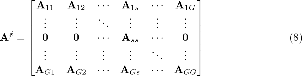
Double counting in the total gross exports of a given country s occurs whenever items that are first exported by s are then reimported and used to produce goods and services to be exported again by country s. Conceptually, one way to distinguish between value added and double counting is to split the production chain in phases, each one delimited by an export flow of country s: what is generated within that particular production phase is accounted for as value added in exports; what comes from further upstream production stages is double counted. This can be implemented in a general ICIO framework by modifying the matrix B in such a way that we can slice down the production process along the outward boundaries of the exporting country s. To this end, consider the representation of the global Leontief inverse as a sum of infinite series of the gross output generated in all upstream stages of the production process:

$B=I+A+A^2+A^3+\cdots +A^n\hspace{1em}n\to \infty$

7

We can split the production process along country s’s borders by carving out its intermediate export linkages at any stage of the above series. Algebraically, it can be implemented by setting to 0 the coefficients of matrix A that identify the direct requirement of intermediate inputs from country s (that is, A _sj = 0 ∀ j ≠ s):

$A^{\cancel{s}}=\left[\begin{array}{cccccc}{A}_{11}& A_{12}& \cdots & A_{1s}& \cdots & A_{1G}\\ ⋮& ⋮& \ddots & ⋮& ⋮& ⋮\\ 0& 0& \cdots & A_{ss}& \cdots & 0\\ ⋮& ⋮& ⋮& ⋮& \ddots & ⋮\\ A_{G1}& A_{G2}& \cdots & A_{Gs}& \cdots & A_{GG}\end{array}\right]$

8

Then the corresponding inverse Leontief matrix is

$B^{\cancel{s}}={\left(I-A^{\cancel{s}}\right)}^{-1}$

9

Given that $B_{is}=B_{is}^{\cancel{s}}+B_{is}^{\cancel{s}}{\displaystyle \sum _{j\ne s}{A}_{sj}}{B}_{js}$ , (6) can be rewritten so that we can single out the value-added and double-counted terms within each component:

$\begin{array}{c}{u}_N{E}_{s*}=\stackrel{\text{domestic content (}D{C}_{s*}\text{)}}{\overbrace{\underset{\begin{array}{c}\text{ domestic value }\\ \text{ added }\\ \left(DV{A}_{s*}\right)\end{array}}{\underbrace{V_s{B}_{ss}^{\cancel{s}}{E}_{s*}}}+\underset{\begin{array}{c}\text{ domestic double }\\ \text{ counted }\\ \left(DD{C}_{s*}\right)\end{array}}{\underbrace{V_s{B}_{ss}^{\cancel{s}}{\displaystyle \sum _{j\ne s}{A}_{sj}}{B}_{js}{E}_{s*}}}}}\\ +\stackrel{\text{foreign content (}F{C}_{s*}\text{)}}{\overbrace{\underset{\begin{array}{c}\text{ foreign value }\\ \text{ added }\\ \left(FV{A}_{s*}\right)\end{array}}{\underbrace{{\displaystyle \sum _{t\ne s}^G{V}_t}{B}_{ts}^{\cancel{s}}{E}_{s*}}}+\underset{\begin{array}{c}\text{ foreign }\\ \text{ foreign double }\\ \text{ counted }\\ \left(FD{C}_{s*}\right)\end{array}}{\underbrace{{\displaystyle \sum _{t\ne s}^G{V}_t}{B}_{ts}^{\cancel{s}}{\displaystyle \sum _{j\ne s}{A}_{sj}}{B}_{js}{E}_{s*}}}}}\end{array}$

10

Equation (10) reproduces the breakdown of bilateral exports into the main items identified in Koopman, Wang, and Wei (2014) (see figure 2). The double-counted items are measured by isolating the portion of country s that has been already exported by s in a previous stage of the production process. As far as the domestic components are concerned, it is worth noting that $B_{ss}^{\cancel{s}}$ corresponds with the so-called local Leontief matrix (I − A _ss ) ^{− 1}. This means that the domestic value added in exports is obtained by isolating all the domestic stages of production needed to produce the exported goods while ignoring the domestic content of imported inputs.¹⁵ The foreign value added in (10) follows the same rationale, that is, considering as value added only the items crossing country s’s border once. ¹⁶

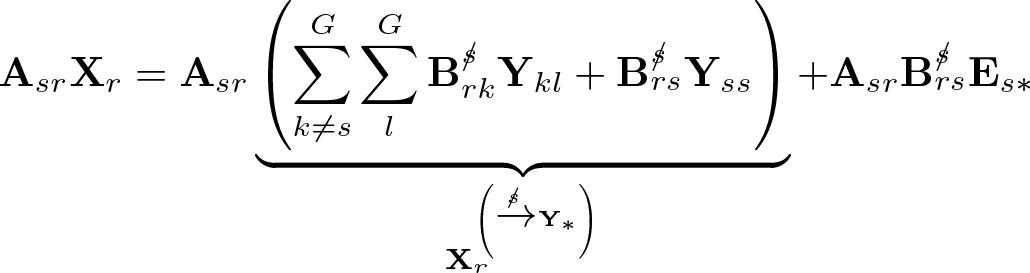
In addition to the breakdown of the value added by country of origin, it is also possible to consider the linkages with the market of final absorption. To this aim, total exports E _s∗ can be split into final goods $\left({\displaystyle {\sum }_{r\ne s}^G{Y}_{sr}}\right)$ and intermediate inputs required by the production of gross output of the importing countries $\left({{\displaystyle \sum }}_{r\ne s}^G{A}_{sr}{X}_r\right)$ .

$E_{s*}={\displaystyle \sum _{r\ne s}^G{Y}_{sr}}+{\displaystyle \sum _{r\ne s}^G{A}_{sr}}{X}_r$

11

Then, intermediate inputs imported by the direct partner (A _sr X _r ) can be followed through the country of final completion and the market of ultimate demand. According to one of the basic IO accounting relations (that is, X = BY), all the remaining (and potentially infinite) stages of production are accounted for by the Leontief inverse matrix B. Finally, the domestic value added (DVA) and the foreign value added (FVA) in the total exports of s can be reexpressed as

$DV{A}_{s*}=V_s{\left(I-A_{ss}\right)}^{-1}\left({\displaystyle \sum _{r\ne s}^G{Y}_{sr}}+{\displaystyle \sum _{r\ne s}^G{A}_{sr}}{\displaystyle \sum _k^G{\displaystyle \sum _l^G{B}_{rk}}}{Y}_{kl}\right)$

12

and

$FV{A}_{s*}={\displaystyle \sum _{t\ne s}^G{V}_t}{B}_{ts}^{\cancel{s}}\left({\displaystyle \sum _{r\ne s}^G{Y}_{sr}}+{\displaystyle \sum _{r\ne s}^G{A}_{sr}}{\displaystyle \sum _k^G{\displaystyle \sum _l^G{B}_{rk}}}{Y}_{kl}\right)$

13

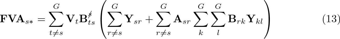
It is worth recalling that the two subscripts on final demand matrix Y refer to the country of final completion and the market of final absorption. ¹⁷ With the icio command, it is possible to single out the markets (and sectors) of final absorption by using the option destination() (see section 4.4). One can also obtain information on specific country–sector of origin of the value added with the option origin(). The details on the sectors of origin or destination are obtained with the same algebraic formulation of matrices V and Y shown in (5).

In addition, to identify specific country–sector of origin or destination from (12) and (13), the domestic value added can be broken down in two main aggregate indicators (see figure 2) to distinguish between the DVA ultimately absorbed in the country of origin s (that is, the “reflection” component in Koopman, Wang, and Wei [2014]; REF _s∗ ) or in a foreign market (that is, the value-added exports, or VAX _s∗ , in Johnson and Noguera [2012] nomenclature):

$\begin{array}{c}RE{F}_{s*}=V_s{\left(I-A_{ss}\right)}^{-1}\left({\displaystyle \sum _{r\ne s}^G{Y}_{sr}}+{\displaystyle \sum _{r\ne s}^G{A}_{sr}}{\displaystyle \sum _k^G{B}_{rk}}{Y}_{ks}\right)\\ VA{X}_{s*}=V_s{\left(I-A_{ss}\right)}^{-1}\left({\displaystyle \sum _{r\ne s}^G{Y}_{sr}}+{\displaystyle \sum _{r\ne s}^G{A}_{sr}}{\displaystyle \sum _k^G{\displaystyle \sum _{l\ne s}^G{B}_{rk}}}{Y}_{kl}\right)\end{array}$

4.2 Conceptual framework: Value-added accounting in bilateral exports

4.2.1 Bilateral perspective

If we are interested in measuring the total value added that crosses a specific bilateral border, for instance, to assess the exposure to tariffs imposed by the bilateral partner, we need an accounting method for value added in bilateral exports that excludes from gross trade figures only the items that are double counted in the same bilateral flow. In other words, the specific bilateral relation represents the perimeter for defining doublecounted flows in gross exports. This matters, for example, when we are interested in singling out the value added crossing a specific border that could be exposed to trade tensions between two countries on each side of the relationship.

By proceeding as for the derivation of the value-added decomposition for aggregate trade flows (see section 4.1), we can modify the input coefficient matrix A to split the production process along the new perimeter and single out the value-added and doublecounted items. While in the exporting-country perspective we set to 0 the coefficients that identify the direct requirement of intermediate inputs from country s to all the other countries, here we only set to 0 the bilateral coefficient matrix A _sr :

$A^{\cancel{sr}}=\left[\begin{array}{ccccccc}{A}_{11}& \cdots & A_{1s}& \cdots & A_{1r}& \cdots & A_{1G}\\ ⋮& ⋮& ⋮& ⋮& ⋮& ⋮& ⋮\\ A_{s1}& \cdots & A_{ss}& \cdots & 0& \cdots & A_{sG}\\ ⋮& ⋮& ⋮& ⋮& ⋮& ⋮& ⋮\\ A_{G1}& \cdots & A_{Gs}& \cdots & A_{Gr}& \cdots & A_{GG}\end{array}\right]$

Then the corresponding inverse Leontief matrix can be defined as

$B^{\cancel{sr}}={\left(I-A^{\cancel{sr}}\right)}^{-1}$

By analogy, with the derivation of the decomposition of aggregate exports in (10),

we can express the complete decomposition of bilateral exports based on a bilateral perspective:

$\begin{array}{l}{u}_N{E}_{sr}=\stackrel{\begin{array}{c}\text{domestic }\\ \text{content (}{\mathbf{DC}}_{sr}\text{)}\end{array}}{\overbrace{\underset{\begin{array}{c}\text{bilateral}\\ \text{perspective}\\ {\mathrm{DVA}}_{sr}^{*}\end{array}}{\underbrace{V_s{B}_{ss}^{\cancel{sr}}{E}_{sr}}}+\underset{\begin{array}{c}\text{bilateral}\\ \text{perspective}\\ {\mathbf{DDC}}_{sr}^{*}\end{array}}{\underbrace{V_s{B}_{ss}^{\cancel{sr}}{A}_{sr}{B}_{rs}{E}_{sr}}}}}+\stackrel{\begin{array}{c}\text{foreign }\\ \text{content (}{\mathbf{FC}}_{sr}\text{)}\end{array}}{\overbrace{\underset{\begin{array}{c}\text{bilateral}\\ \text{perspective}\\ {\mathbf{FVA}}_{sr}^{*}\end{array}}{\underbrace{{\displaystyle \sum _{t\ne s}^G{V}_t}{B}_{ts}^{\cancel{sr}}{E}_{sr}}}+\underset{\begin{array}{c}\text{bilateral}\\ \text{perspective}\\ {\mathbf{FDC}}_{sr}^{*}\end{array}}{\underbrace{{\displaystyle \sum _{t\ne s}^G{V}_t}{B}_{ts}^{\cancel{sr}}{A}_{sr}{B}_{rs}{E}_{sr}}}}}\\ \end{array}$

14

The measures of domestic value added ( ${\mathbf{DVA}}_{sr}^{*}$ ) and foreign value added ( ${\mathbf{FVA}}_{sr}^{*}$ ) in (14) correspond to those proposed by Johnson (2018) in a two-country context; the same measure of domestic value added in bilateral exports is also obtained by Los, Timmer, and de Vries (2016) by using hypothetical extraction.

Similarly to the derivation of (11) to (13), (14) can be further developed to consider all the forward production linkages, as well as the countries of completion and the markets of final absorption.

4.2.2 Exporting-country perspective for bilateral trade flows

The methodology presented above provides a correct measure of the whole value added that crosses a specific bilateral border, but these indicators cannot be summed across bilateral destinations to get the correct aggregate measure; that is, they are not additive. Conversely, to obtain a consistent breakdown across bilateral flows, the exportingcountry perspective must also be applied to the decomposition of disaggregated trade flows.

However, in this case, an approach to allocate value-added and double-counted items across the different disaggregated trade flows is needed. To address this issue, we exploit two alternative approaches proposed by Nagengast and Stehrer (2016) and fully derived by Borin and Mancini (2015, 2017).

The source-based approach is when a given item is accounted for as value added the first time it leaves the country of origin and, in the case of multiple crossings, is considered double counted in subsequent shipments. This definition is in line with the logic behind the accounting procedure presented in (7) through (10). ¹⁸ The sink-based approach is when a given item is accounted for as value added the last time it leaves the country of origin and, in the case of multiple crossings, is considered double counted in prior shipments. Suppose, for instance, that along the production process a certain item is exported by country A first to country B and then to country C. With the source-based approach, the item is classified as value added the first time it crosses the national border (that is, in the exports toward B), whereas the sink-based approach considers it as value added the last time it crosses the border (that is, in the exports toward C).

As already mentioned, the source approach is useful to separate traditional exports (crossing one border) from GVC exports (crossing more than one border). Instead, the sink approach is more suited for the analysis of bilateral trade balances in terms of value added.

The value-added decomposition of the exports from country s to country r according to a source-based approach of the exporting-country perspective can be obtained simply by substituting the total exports of s in (10) with the considered bilateral trade flow (that is, E _sr ):

$\begin{array}{c}{u}_N{E}_{sr}=\stackrel{\begin{array}{c}\text{domestic }\\ \text{content (}{\mathbf{DC}}_{sr}\text{)}\end{array}}{\overbrace{\underset{\begin{array}{c}\text{domestic value}\\ \text{added}\\ \text{(}\mathbf{DVA}\hspace{0.17em}sourc{e}_{sr}\text{)}\end{array}}{\underbrace{V_s{B}_{ss}^{\cancel{sr}}{E}_{sr}}}+\underset{\begin{array}{c}\text{domestic double}\\ \text{counted}\\ \text{(}\mathbf{DDC}\hspace{0.17em}sourc{e}_{sr}\text{)}\end{array}}{\underbrace{V_s{B}_{ss}^{\cancel{sr}}{\displaystyle \sum _{j\ne s}{A}_{sj}{B}_{js}{E}_{sr}}}}}}\\ +\stackrel{\begin{array}{c}\text{foreign }\\ \text{content (}{\mathbf{FC}}_{sr}\text{)}\end{array}}{\overbrace{\underset{\begin{array}{c}\text{foreign value}\\ \text{added}\\ \text{(}\mathbf{FVA}\hspace{0.17em}sourc{e}_{sr}\text{)}\end{array}}{\underbrace{{\displaystyle \sum _{t\ne s}^G{V}_t}{B}_{ts}^{\cancel{sr}}{E}_{sr}}}+\underset{\begin{array}{c}\text{foreign double}\\ \text{counted}\\ \text{(}\mathbf{FDC}\hspace{0.17em}sourc{e}_{sr}\text{)}\end{array}}{\underbrace{{\displaystyle \sum _{t\ne s}^G{V}_t}{B}_{ts}^{\cancel{sr}}{\displaystyle \sum _{j\ne s}{A}_{sj}{B}_{js}{E}_{sr}}}}}}\end{array}$

15

As to the value-added decomposition of the exports from country s to country r according to an exporting-country perspective or sink-based approach, it is first necessary to isolate the portion of ultimate shipments within a certain bilateral trade flow.

These “ultimate exports” $\left[E_{sr}^{\left(\stackrel{\cancel{s}}{\to }{Y}_{*}\right)}\right]$ are made up of final goods (Y sr) and intermediate goods that do not reenter country s’s exports before reaching the ultimate destination $\left[A_{sr}{X}_r^{\left(\stackrel{\cancel{s}}{\to }{Y}_{*}\right)}\right]$ . Because the latter are commensurate with final goods as concerns the exporting country s, the overall value added can be computed by premultiplying the vector of ultimate exports by the VB matrix (that is, in the same way as how the VBY matrix is used to measure the total value added in final demand in section 3.1). To single out the value-added and double-counted components in the exports of intermediates of country s according to a sink-based approach of the exporting-country perspective, we can use the same algebraic device presented in (9) that allows one to distinguish between the items reexported by s and those that are not. ¹⁹

$A_{sr}{X}_r=A_{sr}\underset{X_r{ }^{\left(\stackrel{\cancel{s}}{\to }{Y}_{*}\right)}}{\underbrace{\left({\displaystyle \sum _{k\ne s}^G{\displaystyle \sum _l^G{B}_{rk}^{\cancel{s}}}}{Y}_{kl}+B_{rs}^{\cancel{s}}{Y}_{ss}\right)}}+A_{sr}{B}_{rs}^{\cancel{s}}{E}_{s*}$

Then the value-added breakdown of bilateral exports can be expressed as

$\begin{array}{l}{u}_N{E}_{sr}=\stackrel{\begin{array}{c}\text{domestic}\\ \text{content (}{\mathbf{DC}}_{sr}\text{)}\end{array}}{\overbrace{V\underset{\begin{array}{c}\text{domestic double}\\ \text{added (}\mathbf{DVA}sin{k}_{sr}\text{)}\end{array}}{\underbrace{{ }_s{B}_{ss}\left\{Y_{sr}+A_{sr}\left({\displaystyle \sum _{k\ne s}^G{\displaystyle \sum _l^G{B}_{rk}^{\cancel{s}}}}{Y}_{kl}+B_{rs}^{\cancel{s}}{Y}_{ss}\right)\right\}}}+\underset{\begin{array}{c}\text{domestic double}\\ \text{counted (}\mathbf{DDC}sin{k}_{sr}\text{)}\end{array}}{\underbrace{V_s{B}_{ss}{A}_{sr}{B}_{rs}^{\cancel{s}}{E}_{s*}}}}}\\ +\stackrel{\begin{array}{c}\text{foreign}\\ \text{content (}{\mathbf{DC}}_{sr}\text{)}\end{array}}{\overbrace{\underset{\begin{array}{c}\text{foreign double}\\ \text{added (}\mathbf{FVA}sin{k}_{sr}\text{)}\end{array}}{\underbrace{{\displaystyle \sum _{t\ne s}^G{V}_t}{B}_{ts}\left\{Y_{sr}+A_{sr}\left({\displaystyle \sum _{k\ne s}^G{\displaystyle \sum _l^G{B}_{rk}^{\cancel{s}}}}{Y}_{kl}+B_{rs}^{\cancel{s}}{Y}_{ss}\right)\right\}}}+\underset{\begin{array}{c}\text{foreign double}\\ \text{counted (}\mathbf{FDC}sin{k}_{sr}\text{)}\end{array}}{\underbrace{{\displaystyle \sum _{t\ne s}^G{V}_t}{B}_{ts}{A}_{sr}{B}_{rs}^{\cancel{s}}{E}_{s*}}}}}\\ \end{array}$

16

As highlighted above, the three different value-added decompositions of bilateral trade flows in (14), (15), and (16) can be used to address different issues, for instance, the analysis of the exposure to tariffs imposed by the bilateral partner, the analysis of GVC exports, and the analysis of bilateral trade balances, respectively. Nevertheless, it is important to highlight that (i) at the bilateral level, the domestic and foreign contents are the same in the three breakdowns, and only the value-added and doublecounted components differ; and (ii) the value-added and double-counted terms of the two decompositions based on the exporting-country perspective [that is, the source-based perspective in (15) and the sink-based perspective in (16)] differ only at the bilateral level, and when summing across the destinations of a given exporter, we obtain exactly the same aggregate indicators as those in (10). ²⁰

4.3 Conceptual framework: Value-added accounting in different types of trade flows and accounting perspectives

Here we provide an overview of all the trade flows that can be analyzed with icio, with the corresponding perspectives that are available.

• 1. Total exports of a country

• - World perspective: This perspective has been considered only for the decomposition of the foreign content of exports. According to this methodology, a certain item is accounted for as foreign value added only once in all (that is, world) trade flows, whereas in the exporting-country perspective it occurs only once in all the exports of a single country. More specifically, by using a source-based (sink-based) approach, a certain item is considered as value added only the first (the last) time it crosses a foreign border, whereas all the other times it does, it is classified as double counted. The decompositions based on a world perspective can be used to address interesting questions regarding the breakdown of total world trade (by aggregating across countries the total exports’ decompositions obtained with icio). For instance, we can measure the share of world’s GDP entering the exports of some other country. However, these measures are usually unsuited to addressing relevant issues regarding a country’s exports. ²¹

b. Total sectoral exports

- Sectoral-exporter perspective: This method, formally derived in Borin and Mancini (2019), can be chosen when the aim of the analysis is to compute the entire value added that is embedded in all the exports of a country in a given sector. This occurs, for instance, when an economic shock (or policy intervention) affects all the exports of a country in a given sector (across all the destinations), and the interest of the analyst is to measure the spillovers from this shock into different country sectors. The domestic and foreign value added embedded in total exports of country s and sector n can be computed similarly as in the decomposition of bilateral flows according to the bilateral perspective [see (14)]. The only difference is that the original matrix of technical coefficients A needs to be modified such that a_sj,n is set to 0 ∀ j ≠ s; thus, the inverse Leontief matrix is computed accordingly.

- Exporting-country perspective: This accounting method for the analysis of sectoral trade flows follows exactly the logic of the same perspective described above for the analysis of bilateral trade flows. It provides a breakdown of sectoral exports consistent with the value-added indicators computed for the total aggregate exports of a country. Depending on whether the focus of the analysis is on the origin of the production or on the final absorption, a source- or a sink-based approach needs to be considered, respectively. The algebraic expressions follow closely the formulas in (10) [or (15)] and (16), where total sectoral export flows are singled out through proper diagonalizations of the VB and the $V{B}^{\cancel{s}}$ matrices. ²²

2. Bilateral exports of a country

a. Bilateral aggregate exports: Both the logic and the algebraic formulation of these accounting perspectives are presented in section 4.2.

- Bilateral perspective

- Exporting-country perspective

b. Bilateral sectoral exports:

- Sectoral-bilateral perspective: This methodology, developed in Borin and Mancini (2019), is useful for empirical analysis aiming to measure the whole value added of a country entering in the exports of country s in a specific sector (say, n) to an importing country r. It can be used, for instance, to evaluate the GDP exposure to a tariff imposed by a country vis-à-vis a certain partner in a specific sector. As for the previous decompositions, for which the perspective corresponds to the trade flow under investigation, the value-added indicators are derived by modifying the input requirement matrix A, setting to 0 all the coefficients corresponding to the intermediate exports from s to r in (exporting) sector n.

- Exporting-country perspective: This can be used to obtain a breakdown of total exports’ value-added indicators across sectoral-bilateral flows. The formulation is a direct extension of that used for total sectoral exports to bilateral trade flows.

3. Total imports of a country

a. Total aggregate imports:

- Importing-country perspective: This methodology can be exploited to compute the GDP of a given country j that enters, directly or indirectly, in the total imports of a given country r. This measure is interesting, for instance, when a certain country is going to adopt a general protectionist stance (that is, vis-à-vis all the exporting partners) and we want to compute the portion of the other countries’ GDP at stake. In this case, we define the relevant perimeter at the level of the importing country’s borders as a whole. This can be implemented by following a procedure similar to that used to derive the (exporting) country perspective of section 4.1 and is formally derived in Borin and Mancini (2019).

b. Total sectoral imports:

- Sectoral-importer perspective: This perspective, derived in Borin and Mancini (2019), can be useful when the focus is on a particular sector of a given importing country, for example, when a certain shock affects only the imports of a country in a specific sector. The derivation is similar to that of the importing-country perspective, where the double-counting perimeter is defined at the level of the sectoral imports of a country.

4.4 Implementation: Accounting for value added in gross trade

Depending on the specific empirical question, the user needs to choose the appropriate icio options to select i) the desired trade flow, ii) the best-suited accounting methodology to single out double-counted components (see above for a definition of double counting), and iii) the appropriate results to retrieve.

As to the first point, the following types of trade flows are considered: i) aggregate exports, ii) sectoral exports, iii) bilateral exports, iv) sectoral-bilateral exports, v) aggregate imports, and vi) sectoral imports. It is also worth recalling that the option group() allows the user to consider value-added decompositions for country aggregates so that the set of trade flow combinations is actually broader (see section 3.2.3 for examples). For each trade flow, we consider the accounting perspectives and approaches that appear to be more economically important (see section 4.3 for an overview).

4.4.1 Syntax

We structured icio‘s syntax according to the different trade flows as follows:

• 1. Value added and GVC participation in total exports of a country:

• b. Value added and GVC participation in total sectoral exports:

  icio, exporter( country_code [ , sector_code ] ) [ methods_1b ] [ results_exports ] [ origin_destination ] [ standard_options ]

• 2. Value added and GVC participation in bilateral exports:

• b. Value added and GVC participation in bilateral sectoral exports:

  icio, exporter(country_code [ , sector_code ] ) importer(country_code) [ methods_2b ] [ results_exports ] [ origin_destination ] [ standard_options ]

• 3. Value added in total imports of a country:

• b. Value added in total sectoral imports:

  icio, importer(country_code [ , sector_code ] ) [ method_3b ] [ results_imports ] [ origin_destination ] [ standard_options ]

4.4.2 methods_* options

The options perspective() and approach() can be used to select the appropriate accounting methodology (that is, [ methods_* ] in the syntax reported above) for answering the empirical question of interest. The rationale and the algebraic formulation of the different accounting methodologies have been discussed in previous sections. For the different trade flows, table 3 reports a summary of the available perspectives.

Table 3.

A summary of the available perspectives and approaches for each trade flow: Syntax

	Perspective in line with the trade flow	Perspective consistent with more aggregate flows (that is, additive)
1. Total exports 1a. Aggregate methods_1a 1b. Sectoral methods_1b	perspective(exporter) perspective(sectexp)	perspective(world) approach(source) perspective(world) approach(sink) perspective(exporter) approach(source) perspective(exporter) approach(sink)
2. Bilateral exports 2a. Aggregate methods_2a 2b. Sectoral methods_2b	perspective(bilateral) perspective(sectbil)	perspective(exporter) approach(source) perspective(exporter) approach(sink) perspective(exporter) approach(source) perspective(exporter) approach(sink)
3. Total imports 3a. Aggregate method_3a 3b. Sectoral method_3b	perspective(importer) perspective(sectimp)	not applicable not applicable

As already mentioned at the beginning of section 4, whenever the perspective is set at a more aggregate level compared with the considered trade flow, two alternative approaches are available. By using the icio option approach(source), the item is classified as value added the first time it crosses the national border, whereas the option approach(sink) considers it as value added the last time it crosses the border.

4.4.3 results_exports and results_imports options

For the selected trade flow, icio allows one to compute the main indicators of gross trade and value-added trade through the return() option. ²³

For export flows (that is, [results_exports] in the syntax reported at the beginning of this section), the default output is return(detailed). It allows one to get a complete value-added decomposition of the trade flows according to the conceptual scheme of figure 2 in section 4.1. Gross trade (gtrade) is split into the part that is originally produced by the exporting country (domestic content—dc) and the part that is produced abroad (foreign content—fc); in turn, each of these components is broken up into part value-added item (domestic value added—dva—and foreign value added—fva) and part double counting. ²⁴ The methodology used to single out the value-added and double-counted components changes according to the selected perspective and approach options, while the gtrade, dc, and fc measures are, by construction, the same regardless of the accounting methodology.

The detailed output also includes additional indicators of trade in value added that have been singled out in the literature (for example, VAX by Johnson and Noguera [2012]; reflection by Koopman, Wang, and Wei [2014]; and DAVAX and VAXIM by Borin and Mancini [2019]; see section 4.1 for an overview) and also measures of GVC participation ²⁵ as developed in Borin and Mancini (2015, 2019). The additional indicators that are included in the detailed output vary consistently with the selected perspective and approach options. The user can also ask for a specific trade indicator by specifying one of the following arguments of the return() option: gtrade, dc, dva, fc, or fva. ²⁶

As far as import flows are concerned (that is, [results_imports] in the syntax reported at the beginning of this section), the distinction between domestic and foreign items is less relevant because the former would refer only to the items produced, exported, and then reimported by the importing country itself. For this reason, the default in this case is to compute the gross trade value (that is, gtrade); the value added (that is, va) can also be retrieved. For the analysis of import flows, it might also be useful to specify an origin or destination of the gross content or value added, as highlighted in the next paragraph.

4.4.4 origin_destination option

As an additional feature, it is also possible to single out the country–sector where the goods and services were originally produced by specifying the origin(country_code [ , sector_code ] ) option, as well as the market–sector where they are absorbed in the final demand, by specifying the destination(country_code [ , sector_code ] ) option (that is, [origin_destination] in the syntax reported at the beginning of this section). Results for all countries or all sectors can be computed and displayed simultaneously, using all as the argument for country_code or sector_code (both cannot be all at once). If the aim is to compute the value added produced by a specific country–sector of origin, the option return(va) must be specified. ²⁷ The gross content term (that is, value added + double-counted items) for a specific country (and sector) of origin can be computed by specifying return(gtrade).

Similarly, the imported value added (gross content) can be traced back to the country of origin by specifying the option origin(country_code [ , sector_code ] ) together with return(va) (return(gtrade)). Of special note is that it is possible to also pin down a specific market–sector of final demand by specifying the destination(country_code [ , sector_code ] ) option.

4.4.5 standard_options

As for the standard options, (that is, [ standard_options ] in the syntax reported at the beginning of this section), the save() and group() options are available for both export and import flows (see section 3.2 for a description of these options).

4.4.6 Examples: Value added in trade flows

In this section, we provide some examples of the insights that icio, dealing with the breakdown of value added in trade flows, can bring for the economic analysis of ICIO tables.

As a running example, we select a specific trade flow, the Chinese total aggregate exports. After loading the year 2014 of the last release of the WIOD tables by using

. icio_load, iciotable(wiodn) year(2014)

the user can easily obtain a detailed breakdown of the selected trade flow, both in millions of U.S. dollars and as a share, by using

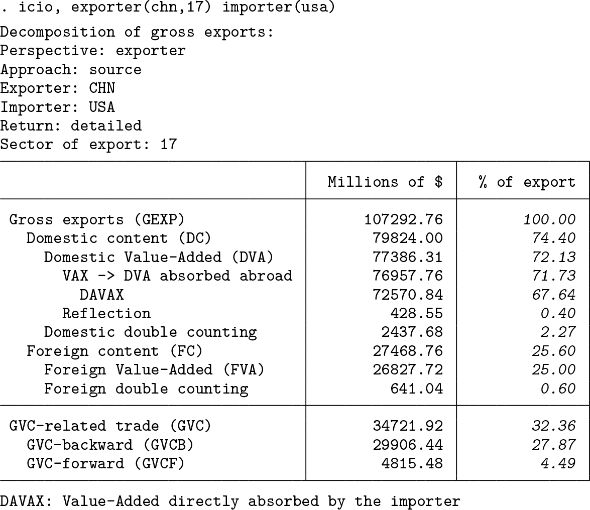
The detailed decomposition also can be computed for a particular sector of export, for example, “Manufacture of computer, electronic, and optical products” (sector code 17 for the loaded ICIO table), by using ²⁸

We now show how the results can change by using a different perspective on the same trade flow. We move from the default—the exporting-country perspective—to a sectoral-exporter perspective by adding the option perspective(sectexp).

While the output confirms that domestic and foreign contents are not affected by changing perspective, the value-added terms are higher, and consequently, doublecounting items are lower. This is not surprising, because the sectoral-exporter perspective features a more restrictive definition of double counting (see section 4.3).

Which perspective should be used? It depends on the specific empirical question. If the goal is to measure to what extent the GDP of a country could be exposed to a certain shock on the exports of a sector, a sectoral-exporter perspective might be appropriate. Indeed, in this case, the relevant border to trace value added belongs to the exporting country–sector pair. Instead, the default perspective (the exporting-country one) is the most appropriate if the goal is to compute GVC-related trade indices—because to this end the relevant border is always the exporting country’s border—and is suited to obtain measures of value-added trade traced in disaggregated trade flows that are consistent with the aggregate figures. This additivity property is a feature of the exporting-country perspective only. ²⁹ It can be easily verified by showing that value-added components and GVC-related trade in the aggregate Chinese exports—as computed before using the syntax icio, exporter(chn)—equal the sum of the same measures obtained for each sector. A possible implementation of this check is the following:

We now select a different trade flow, moving to bilateral sectoral exports. In particular, we consider the Chinese exports of computer, electronic, and optical products to the U.S. The default assessment of the extent of GVC participation, as well as a breakdown of the flow in terms of value-added components consistent both with the aggregate Chinese exports and with total Chinese exports to the U.S. is obtained using the default exporting-country perspective:

Again, we can select a perspective in line with the level of aggregation of the chosen trade flow, that is, a sectoral-bilateral perspective—perspective(sectbil), for instance, to measure the extent to which the Chinese GDP could be exposed to a tariff imposed by the U.S. on the imports of computer, electronic, and optical products:

According to WIOD 2014 data, Chinese value added potentially exposed to this tariff turned out to be around $79.8 billion, as shown by the value reported for the Domestic Value-Added (DVA). This is higher than the $77.4 billion of Chinese value added traced in the same export flow using an exporting-country perspective (see the previous icio output above). Thus, if we had used the latter perspective, we would have understated the Chinese exposure. Again, each empirical question calls for the best-suited perspective: the default exporting-country perspective is more useful if the aim is to assess GVC participation or to retrieve measures of value-added trade consistent with the figures at a more aggregate level; the perspective in line with the selected trade flow is more suited to encompass the entire value added that might be affected by a shock hitting that particular flow.

The same reasoning applies when the objective is to choose the best-suited perspective for bilateral aggregate exports. Here the choice will be, again, between the default exporting-country perspective and the bilateral one. For example, suppose that the aim is to quantify the potential exposure of other countries to a U.S.–China trade war. In fact, U.S. and Chinese exports embed a nonnegligible amount of other countries’ foreign value added that would be indirectly exposed to new tariffs. Figure 4.9 of the World Bank’s WDR 2020 reports that around 2% of the value added in the Chinese exports to the U.S. consists of Japan’s GDP. In turn, around 2.6% of the value added in the U.S. exports to China is Canadian GDP. These numbers can be easily obtained using icio by selecting a bilateral perspective and retrieving the value added by country of origin in a particular bilateral flow. In fact, the value added that crosses the specific bilateral border where the new tariffs could be in place, that is, the GDP potentially affected by trade barriers, can be computed using the following syntax:

In the above Stata output, we retrieved only the exposure for countries with the highest value added in the bilateral exports between U.S. and China. Actually, by running the previous syntax with the option origin(all), icio would report the results for each country in the Eora database. Because the complete list is very long, the user may find it useful to exploit the save() option. As shown below, by adding this option, the complete icio output can be saved into a file called wdr_4_9.xlsx, in the sheets A and B, within the current working directory

Finally, we consider the analysis of value added in the total imports of a country. To quantify the German GDP potentially exposed to U.S. tariffs vis-à-vis all partners, according to WIOD 2014 data, we can use the following syntax:

The Stata output indicates that around $133 billion of Germany’s value added is imported, directly and indirectly, by the U.S. (around 5.5% of the total U.S. imports) and thus could be exposed to U.S. trade barriers, according to WIOD 2014 data. German GDP exposure to these trade barriers can be computed by taking the ratio with respect to the total German GDP—obtained with icio, origin(deu). Thus, around 3.7% of German GDP could be affected by these U.S. trade barriers. In a GVC world, the GDP exposure to a trade barrier could be direct—through the country’s exports to the economy that has imposed the trade restrictive measure—or indirect—through the exports of other countries. The former can be computed by looking at the German GDP directly exported to the U.S., via this command: icio, origin(deu) exporter(deu) importer(usa) perspective(bilateral) return(va). Thus, 2.8% of German GDP could be directly affected by U.S. tariffs, while 0.9% could be affected through other countries’ exports to the U.S. of German products.

If the goal is to quantify the potential exposure of German value added to a U.S. tariff on a specific sector, for example, motor vehicles from Germany, a sectoral-importer perspective is the right choice.

Again, the relative exposure can be easily obtained by taking the ratio of the absolute exposure ($17.2 billion) with respect to the total German value added in the motor vehicles industry ($147.5 billion). Thus, a U.S. tariff hitting motor vehicle imports from Germany might affect around 11.7% of the value added produced in the same sector in Germany.

Other examples of questions that could be answered using icio for the analysis of value-added trade are the following:

• Which part of a country’s total exports is home produced, that is, domestic GDP?

  icio, exporter(deu) return(dva)

• Which part of a country’s total exports can be traced back to other countries’ GDP?

  icio, exporter(deu) return(fva)

• Where is the foreign value added in German exports produced?

  icio, origin(all) exporter(deu) return(fva)

• Considering the bilateral exports from Italy to Germany, where is the Italian GDP (domestic value added) reexported by Germany absorbed?

  icio, exporter(ita) importer(deu) destination(all) return(dva)

• How can the complete breakdown by origin and destination of the value added (both domestic and foreign) for Chinese exports to the U.S. be obtained?

  icio, origin(all) exporter(chn) importer(usa) /// destination(all) return(va) save(CHN_to_USA)

• How can the (corrected) Koopman, Wang, and Wei (2014) decomposition be retrieved using icio?

  icio, exporter(deu) perspective(world) approach(sink)

• What is the Chinese GDP that at any point in time passes through a certain bilateral trade flow, say, Chinese exports to the U.S.? In other terms, what is the Chinese GDP potentially exposed to U.S. tariffs on imports from China?

  icio, exporter(chn) importer(usa) perspective(bilateral) /// return(dva)

• What is the German GDP potentially exposed to U.S. trade barriers on all imports?

  icio, origin(deu) importer(usa) perspective(importer) return(va)

• What is the German GDP that could be affected by U.S. tariffs on imports in sector 20?

  icio, origin(deu) importer(usa,20) perspective(sectimp) return(va)

• What is the exposure of U.S. GDP to a Chinese tariff on U.S. imports in sector 17?

  icio, exporter(usa,17) importer(chn) perspective(sectbil) /// return(dva)

• To what extent are Italian sectors exposed to a shock on Germany’s exports in sector 20?

  icio, origin(ita,all) exporter(deu,20) perspective(sectexp) /// return(va)

5 Measuring GVC-related exports

Following the original idea by Hummels, Ishii, and Yi (2001), many contributions in the literature have shared the view that the trade flow related to GVC activity should consist of goods and services crossing more than one border along the production process. Borin and Mancini (2015) made this definition operational by proposing a way to isolate traditional trade from gross flows (that is, the portion of trade crossing just one border) and considering the remaining part as a proxy of the GVC-related trade. This GVC indicator presents three desirable features: (i) it is bounded between 0 and 1 because it traces within a particular trade flow its share related to GVC activity; that is, the numerator is a subcomponent of the denominator; (ii) it is additive at any level of aggregation or disaggregation of trade flows; thus, data can be summed at any level (total country exports/world exports/world sector exports/country groups) to obtain the proper GVC participation measures at the desired level of aggregation; and (iii) it can be broken down into two additive terms, that is, a “backward” component corresponding to import content of exports and a “forward” component, which measures the part of domestic production that is supplied to the importing country to be processed and reexported.

In section 5.1, we provide its conceptual framework, and in section 5.2 we show how to compute GVC measures in icio and present some examples.

5.1 Conceptual framework: GVC participation

The traditional exports of country s to country r can be defined as the production of s that is directly absorbed in r without any further reexport. This component, called DAVAX—that is, directly absorbed value added in exports—can be computed as

$DAVA{X}_{sr}=V_s{(I-A_{ss})}^{-}{ }^1{Y}_{sr}+V_s{(I-A_{ss})}^{-}{ }^1{A}_{sr}{(I-A_{rr})}^{-}{ }^1{Y}_{rr}$

Then, GVC-related exports can be simply obtained by excluding the entire domestic

value added of country s absorbed directly by its direct importer (DAVAX _sr ) from its exports to r:

$GVC{X}_{sr}=u_N{E}_{sr}-DAVA{X}_{sr}$

Therefore, GVC-related trade share in total exports is given by

$GV{C}_{sr}=\frac{GVC{X}_{sr}}{u_N{E}_{sr}}$

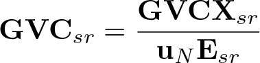
where u _N E _sr is the total exports of country s to country r.

For the total exports of country s, the GVC share will be computed as

$GV{C}_s=\frac{{\displaystyle {\sum }_{r\ne s}^{G}GVC{X}_{sr}}}{u_N{E}_{s*}}$

17

while at world level, we have

$GV{C}_{\text{world }}=\frac{{\displaystyle {\sum }_s^G{\displaystyle {\sum }_{r\ne s}^{G}GVC{X}_{sr}}}}{{\displaystyle {\sum }_s^G\left(u_N{E}_{s*}\right)}}$

As already mentioned, the overall GVC indicator of (17) can be decomposed into a backward component, corresponding to the VS Index proposed by Hummels, Ishii, and Yi (2001) (see Borin and Mancini [2019] for a formal proof) and a forward component, that is, the part of domestic production that is supplied to the importing country to be reexported:

$GV{C}_{sr}=GVC{\text{ backward }}_{sr}+GVC{\text{ forward }}_{sr}$

where

$GVC{\text{ backward}}_{sr}=\frac{V_s{\left(I-A_{ss}\right)}^{-1}{\displaystyle \sum _{j\ne s}^G{A}_{sj}}{B}_{js}{E}_{sr}+{\displaystyle \sum _{t\ne s}^G{V}_t}{B}_{ts}{E}_{sr}}{u_N{E}_{sr}}$

and

$GVC{\text{ forward}}_{sr}=\frac{V_s{\left(I-A_{ss}\right)}^{-1}{A}_{sr}{\left(I-A_{rr}\right)}^{-1}\left({\displaystyle \sum _{j\ne r}^G{Y}_{rj}}+{\displaystyle \sum _{j\ne r}^G{A}_{rj}}{\displaystyle \sum _k^G{\displaystyle \sum _l^G{B}_{jk}}}{Y}_{kl}\right)}{u_N{E}_{sr}}$

The GVC forward _sr indicator differs from the VS1 _s index proposed by Koopman, Wang, and Wei (2014). VS1 _s is computed by aggregating the content of a country’s production embedded in other countries’ exports, and thus it is not necessarily a portion of country s’s exports (like VS). Suppose, for instance, that a certain intermediate component exported by country s later undergoes other processing phases in different countries; the original component will be double counted several times in the summation of country s’s content in other countries’ exports. The discrepancy between the original value of goods exported by s and the related amount that enters in Koopman, Wang, and Wei (2014)’s indicator increases with the relative “upstreamness” of country s’s production.

5.2 Implementation: GVC in exports

To compute GVC measures with icio, the user needs to select (i) the desired trade flow and (ii) the appropriate GVC measure to be computed (overall, backward, or forward participation). The option perspective(exporter) is imposed in this case because only this perspective allows the distinction between the value of trade crossing just one border and the value of trade further reexported, that is, GVC trade.

5.2.1 Syntax

The icio syntax for the different export flows is the following:

• 1. GVC participation in total exports of a country:

• b. GVC participation in total sectoral exports:

  icio, exporter(country_code [, sector_code ] )[ results_gvc ] [ origin_destination ] [ standard_options ]

• 2. GVC participation in bilateral exports:

• b. GVC participation in bilateral sectoral exports:

  icio, exporter(country_code [ , sector_code ] ) importer(country_code) [ results_gvc ] [ origin_destination ] [ standard_options ]

The return() option, that is, results_gvc in the reported syntax, allows the user to get different measures of GVC-related trade by specifying gvc, gvcb, and gvcf as arguments for total, backward, and forward GVC indicators, respectively. As can be noted from the icio results reported in section 4.4.6, GVC-related indicators are routinely reported as part of the detailed output, when an export flow—at any level of aggregation—is specified.

Also for GVC indicators, it is possible to single out the country–sector where the goods and services were originally produced by specifying the origin(country_code [ , sector_code ] ) option, as well as the country–sector where the goods and services are absorbed in final demand by specifying the destination(country_code [ , sector_code ] ) option.

5.2.2 Examples: GVC-related exports

Imagine that the goal is to compute the GVC-related trade in the agrifood–sector (sector 4 in Eora), as in figure 1.13, panel b of the World Bank’s WDR 2020. For instance, in the case of Tanzania, one of the Sub-Saharan African countries that experienced a significant increase in GVC participation in that sector, the results for 1990 and 2015 can be obtained with the following code:

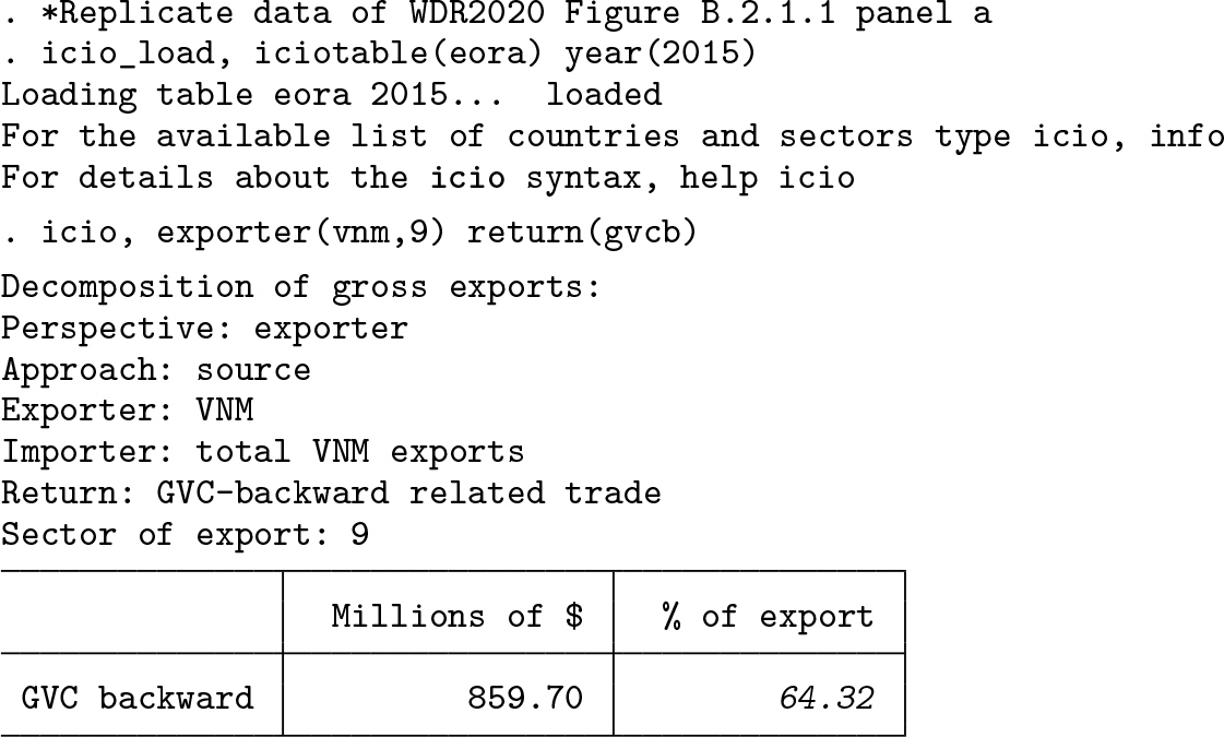
If we want to compute just the backward participation in GVC, for instance, for Vietnam in the electrical and machinery–sector, as in figure B.2.1.1, panel a of the WDR 2020, we can run the following code:

Throughout the WDR 2020, several figures on GVC-related trade at the world level are reported. These measures can be obtained with icio retrieving and then summing the GVC-related trade of each country in the loaded input–output table. Because this could be computationally intensive, we have also released a dataset with GVC indicators and the most relevant measures of value added in trade flows computed for any country– sector for each database available in icio. This database is available on the official WDR 2020 website in the data section. ³⁰

Other basic examples of questions on GVC participation and the related syntax are the following:

• Which share of the German exports related to GVC is produced in Italy?

  icio, origin(ita) exporter(deu) return(gvc)

• Which share of the German exports is related to backward and forward GVC?

  icio, exporter(deu) return(gvcb)

icio, exporter(deu) return(gvcf)

6 Conclusion

In this article, we described the new command, icio, for value-added trade and GVC analysis. Its most important features are the following:

• It exploits the most famous ICIO tables—the WIOD (Timmer et al. 2015), the OECD TiVA Database (OECD 2018), the Eora Global Supply Chain Database (Lenzen et al. 2013), and the ADB MRIOT Database—but also allows one to load any user-provided ICIO table.

• It provides breakdowns of aggregate, bilateral, and sectoral exports and imports according to the source and the destination of their value-added content, with a careful treatment of double-counted items. These decompositions can be used to

• get indicators for any level of disaggregation of trade flows that are consistent with more aggregate measures; that is, disaggregated indicators can be summed up to get correct measures in more aggregate trade flows.

• It can break down export flows in terms of traditional versus GVC trade, at any level of aggregation, also distinguishing between backward and forward participation in GVC.

• It is flexible and open because we plan to release updates to include new ICIO databases as soon as they became available, as well as other measures to assess the participation and position of countries and sectors in GVCs and trade policy analysis.

The measures computed with icio, like any other measure obtained from ICIO tables, suffer from some limitations (Antràs 2020). In fact, ICIO tables are built under strong proportionality assumptions; that is, all output within each country industry is built with the same input mix (de Gortari 2019). However, input–output datasets will soon start exploiting custom data to allow for more heterogeneity in production and trade (United Nations 2018). Once ICIO tables become more detailed, value-added trade measures obtained with the different perspectives featured in icio will diverge more and more, making it even more important to have available the best-suited accounting framework to answer each specific empirical question.

Supplemental Material

Supplemental Material, sj-zip-1-stj-10.1177_1536867X211045573 - icio: Economic analysis with intercountry input–output tables

Supplemental Material, sj-zip-1-stj-10.1177_1536867X211045573 for icio: Economic analysis with intercountry input–output tables by Federico Belotti, Alessandro Borin and Michele Mancini in The Stata Journal