Sage Journals: Discover world-class research

Abstract

Dominance analysis is a common method applied to statistical models to determine the importance of independent variables. In this article, I describe two community-contributed commands, domin and domme, that can be used to dominance-analyze both independent variables and parameter estimates in Stata estimation commands. I discuss how to compute dominance statistics, provide multiple examples of each command applied to data, and outline how to interpret the results from each data-analytic example. I conclude with computational considerations for users applying larger models.

Keywords

st0645 domin domme dominance analysis relative importance analysis decomposition Shapley value decomposition

1 Introduction

Determining the relative importance of independent variables (IVs) in a statistical model has been a subject of study by statisticians and research methodologists for decades (see Budescu and Azen [2004] and Johnson and LeBreton [2004] for reviews of the literature). In many scientific fields, an increasingly common method for determining relative importance is to assess the extent to which an IV reduces prediction error in a statistical model (Budescu 1993; Grömping 2007). Whereas examining the importance of IVs is most common, examining the importance of individual parameter estimates (PEs) in a statistical model is a similar question and another subject of interest to scientists (Luchman, Lei, and Kaplan 2020).

In this article, I discuss two community-contributed commands, domin and domme, that can be used to determine the relative importance of IVs as well as individual PEs in myriad statistical models estimable in Stata using the dominance analysis (DA) approach (Budescu 1993). I begin by discussing the concepts underlying DA as well as how to compute and compare dominance statistics to determine relative importance.

2 DA

DA is a relative-importance determination method that is based on computing the reduction in prediction error that is associated with each IV in a statistical model. Insofar as it is inferring relative importance, the method assumes that the IVs considered have nontrivial contributions to prediction error reduction. That is, DA assumes model selection has occurred prior to computing dominance statistics. DA is therefore intended to determine importance on IVs from a selected model and is not intended for modelselection purposes.

To implement DA, one fits a series of nested models from the data and collects their model fit statistics. The nested models fit from the data are those representing all possible combinations of the IVs as included or excluded from estimation. For p IVs, the number of required models is 2 ^p−1.¹ Traditionally, the model fit statistic used for a DA is an R ² or similar metric that represents (the absence of) prediction error in the model relative to a baseline (for example, the model where all IVs are omitted).

After collecting all the necessary fit statistics, DA moves to comparing the marginal contributions to model fit that are associated with each IV. The most stringent importance determinations computed in DA are the complete dominance designations (Budescu and Azen 2004). Complete dominance is designated by comparing the marginal contribution of two IVs to model fit across every possible comparison of other IVs included or excluded from estimation. For example, consider IVs X_v and X_z . Complete dominance is designated for p IVs using the R ² by

X_{v} D X_{z} if 2^{p - 2} = \sum_{j = 1}^{2^{p - 2}} {\begin{array}{l} if R_{X_{v} S 2_{j}}^{2} - R_{S 2_{j}}^{2} > R_{X_{z} S 2_{j}}^{2} - R_{S 2_{j}}^{2} then \\ if R_{X_{v} S 2_{j}}^{2} - R_{S 2_{j}}^{2} \leq R_{X_{z} S 2_{j}}^{2} - R_{S 2_{j}}^{2} then \end{array}

where X_vDX_z indicates that X_v completely dominates X_z and S2 _j is a distinct subset of the p−2 IVs that excludes both X_v and X_z , which can include the null set of no other IVs. Thus, $R_{X_{v} S 2_{j}}^{2}$ is the R ² for the distinct subset of variables S2 _j , which also includes X_v but not X_z , and $R_{S 2_{j}}^{2}$ is the R ² for the same distinct subset of variables S2 _j , which excludes both X_v and X_z . Complete dominance is then designated if, across all 2 ^p ⁻ ² subsets S2 _j , adding X_v results in a larger increment to the fit statistic (that is, R ²) than adding X_z .

Complete dominance is a stringent criterion and, in many data-analytic conditions, complete dominance cannot be determined between two IVs. In such cases, another criterion to determine importance can be used to compare IVs. This second DA criterion begins by averaging the marginal contributions to the fit statistic attributable to an IV within an order—where order refers to the number of IVs in the model. When we again consider IV X_v , for models with i of the p possible IVs included, the within-order average for variable X_v will be

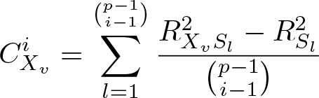
C_{X_{v}}^{i} = \sum_{l = 1}^{(\begin{array}{l} p - 1 \\ i - 1 \end{array})} \frac{R_{X_{v} S_{l}}^{2} - R_{S_{l}}^{2}}{(\begin{matrix} p - 1 \\ i - 1 \end{matrix})}

where S_l is a distinct subset of i−1 IVs that excludes X_v , which can include the null set of no IVs, and $(\begin{matrix} p - 1 \\ i - 1 \end{matrix})$ is the number of distinct combinations of the size of the bottom number (that is, i−1) out of the number of elements of the size of the top number (that is, p−1).

This within-order average is known in DA as a conditional dominance statistic (Budescu 1993). Using the conditional dominance statistic, we can compare each IV’s contributions to model fit and determine a second level of relative importance. Conditional dominance for X_v over X_z is determined when conditional dominance statistics for X_v are bigger than those of X_z across all p orders. Conditional dominance, because of the averaging of the fit statistics within each order and comparing of the resultant averages, is a less stringent criterion for importance than complete dominance.

The most well-known computation in DA is the third criterion that can, in almost every circumstance,² produce an importance determination between two IVs. This third criterion involves taking the within-order averages (that is, conditional dominance statistics, $C_{X_{v}}^{i}$ ) and further averaging them between orders for each IV. Hence, for the p within-order averages or conditional dominance statistics associated with X_v , the between-order average is

C_{X_{v}} = \sum_{i = 1}^{p} \frac{C_{X_{v}}^{i}}{p}

The between-order average of within-order averages is known in DA as a general dominance statistic (Budescu 1993). Similar to the previous two dominance computations, the general dominance statistics can be compared, and a third level of relative importance can be determined. General dominance for X_v over X_z is determined when the general dominance statistic for X_v is bigger than that for X_z . Because it is an average of averages, general dominance is the least stringent criterion for importance compared with complete and conditional dominance. Whereas it is the least stringent, the general dominance statistic is often useful in that it is an additive decomposition (that is, that adds or sums to the total) of the fit statistic into independent components attributable to each IV. In this capacity as a decomposition of a fit statistic, the general dominance statistic is known also as Shapley value decomposition (for example, Grömping [2007]; see also Kolenikov [2000] and Juarez [2012]).

2.1 Extending to PE

To this point, I have been discussing DA only in terms of how IVs contribute to the fit statistic. However, the same logic in terms of ascribing model fit to IVs can also be extended to PEs (see Luchman, Lei, and Kaplan [2020]). In fact, for many statistical models, each IV is represented by a single PE in the model (for example, regress, logit). For models in which an IV might be included in multiple predictive equations (for example, gsem, sureg), being able to disentangle IVs from the PEs that represent them in each prediction equation would be valuable for understanding how such PEs contribute to model fit.

Applying DA to PEs in a multiple-prediction equation model requires a methodology that can isolate a PE within the model, so it can be included or excluded like an IV. Without a method to include or exclude a single PE, all possible combinations of included and excluded PEs from the different models could not be collected for DA statistics and designations.

Excluding an IV for a statistical model like regress is conceptually equivalent to setting its PE to a value of 0; in either case, when one excludes it or sets it to 0, the PE has no effect on prediction. Excluding a PE in a multiple-equation model can then be accomplished by setting the value for that PE to 0. Thus, estimating all possible combinations of PEs included or excluded from a statistical model can be accomplished by mimicking exclusion using value-of-0 constraints. In Stata, models fit using ml often accept the constraints() option. Excluding a PE in such a model is fairly straightforward and can be accomplished by applying null or value-of-0 constraints to PEs to exclude them from prediction. This constraint-based method can be applied to isolate PEs and obtain all combinations of model fit statistics that are included or excluded from the statistical model.

At this point, let me emphasize that DA for PEs using a set of value-of-0 constraints permits many different kinds of models to be evaluated for relative importance—some of which may not make sense conceptually. For example, a user could use PE-based DA to compare error variances with intercepts or means in sem models, but the utility of examining such PEs fit to a log-likelihood-based model fit statistic is likely of questionable value conceptually. Hence, it is incumbent on the user to use the DA to compare PEs that are conceptually reasonable to compare.

Both IV- and PE-based DA have now been introduced, and in the sections below, I transition to introducing two community-contributed commands³ and two wrapper commands designed for the DA of a specific analysis. The first command, domin, can be applied to any statistical model fittable in Stata that follows the standard depvar indepvars format and produces its own fit statistic by default.⁴ This command is generally best suited for IV-based DA. The second command, domme, can be applied to any statistical model fittable in Stata that accepts the constraints() option and can use either a fit statistic returned by the estimation command or one computed using e(ll). This command is focused on PE-based DA but, as will be shown, can be used to obtain IV-based DA as well. The two wrapper commands, mvdom and mixdom, are intended for use with domin and extend its functionality to more complex models. Both wrappers also serve as examples of how to apply domin to official and community-contributed commands that may not fit into domin‘s expected syntax structure or that require the user to compute a fit statistic.

3 IV-based DA: domin

3.1 Command structure

domin can accommodate many statistical models, including regress, logit, poisson, ologit, nbreg, betareg, xtreg, and streg. Again, domin requires that there be a single depvar and a set of indepvars that can be included or excluded individually as varnames from the model.

Syntax

The command syntax is

domin depvar [ indepvars ] [ if ] [ in ] [ weight ] [ , options ]

indepvars cannot include factor variables (see options sets() and all() below, which can) but can include time-series variables for commands in reg() that accept them.

Note that domin requires at least two indepvars or sets of indepvars (see option sets() below). Because it is possible to submit only sets of indepvars, the initial indepvars statement is optional.

aweights, fweights, iweights, and pweights are allowed but must be able to be used by the command in reg(); see [U] 11.1.6 weight.

Options

reg( command , command_options ) is the Stata command or model (that is, the regression) the user intends to apply in the DA. The entry in reg() can be any official command developed by StataCorp, any community-contributed command in the Statistical Software Components (SSC) Archive, or any user-generated command on his or her local machine. The command in reg() must follow the standard single dependent variable model command depvar indepvars syntax. reg() also allows the user to pass command_options for the command in reg(). When a comma is added in reg(), all the syntax following the comma will be passed to each run of the command in reg() as options to that command. reg() is a required option, but when nothing is entered, it defaults to reg(regress) and will produce a warning denoting the default behavior.

fitstat( scalar ) is the scalar-valued model fit statistic used to compute all dominance statistics that are returned by the command in reg(). fitstat() is a required option, but because reg() defaults to reg(regress), the default for this option is fitstat(e(r2)), the R ² scalar returned by regress.

noconditional suppresses the computation and display of conditional dominance statistics. Suppressing the computation of conditional dominance statistics can save computation time when conditional dominance statistics are not desired. Suppressing the computation of conditional dominance statistics also suppresses the “strongest dominance designations” list in the Results window.

nocomplete suppresses the computation of complete dominance designations. Like noconditional, this option suppresses the “strongest dominance designations” list.

epsilon is an approximation to DA using the relative weights analysis or “epsilon” approach (Johnson 2000). epsilon is faster than DA because it does not fit all subsets of possible models but rather uses singular value decomposition to approximate the process.

The epsilon approximation is more limited than the traditional DA approach, allows none of the IV grouping options, and requires noconditional as well as nocomplete. Additionally, epsilon can be used with only three estimation commands currently: regress, glm, and the wrapper program for mvreg discussed below called mvdom.

epsilon obviates each subset regression by orthogonalizing IVs using singular value decomposition (see help matrix svd). epsilon‘s singular value decomposition approach is not equivalent to the all-possible-combinations approach but is many times faster for models with many IVs and tends to produce similar answers regarding relative importance (LeBreton, Ployhart, and Ladd 2004). epsilon also does not allow the use of all(), sets(), mi, consmodel, and reverse and does not allow the use of weights. Using epsilon also produces only general dominance statistics (that is, requires noconditional and nocomplete).

epsilon can obtain general dominance statistics for regress, glm (for any link() and family(), see Tonidandel and LeBreton [2010]) and mvdom (the communitycontributed wrapper program for multivariate regression; see LeBreton and Tonidandel [2008]). By default, epsilon assumes reg(regress) and fitstat(e(r2)). Note that epsilon ignores entries in fitstat() because it produces its own fit statistic.

Note: The epsilon approach has been criticized for being conceptually flawed and biased (see Thomas et al. [2014]), despite research showing similarity between dominanceand epsilon-based methods (for example, LeBreton, Ployhart, and Ladd [2004]). Thus, the user is cautioned in the use of epsilon because its speed may come at the cost of bias.

sets(( indepvars_set ₁ ) … ( indepvars_set_n )) binds together IVs as an inseparable set in the DA. Hence, all IVs in a set will always appear together in a model and are treated as a single IV for dominance statistics computations. Factor and time-series variables can be included in any indepvars_set for commands that accept them.

The user can specify as many IV sets of arbitrary size as is desired. The basic syntax is sets(( x1 x2 ) ( x3 x4 )), which will create two sets (denoted set1 and set2 in the output). set1 will be created from the variables x1 and x2, whereas set2 will be created from the variables x3 and x4. All sets must be bound by parentheses—thus, each set must begin with a left parenthesis, (, and end with a right parenthesis, ), and all parentheses separating sets in the sets() option syntax must be separated by at least one space.

The sets() option is useful for obtaining dominance statistics for IVs that are more interpretable when combined, such as several dummy or effects codes reflecting mutually exclusive groups.

all( indepvars_all ) defines a collection of IVs to be included in all the combinations of models in the DA. The magnitude of the overall fit statistic associated with the set of IVs in the all() option is subtracted from the dominance statistics for all IVs and is reported separately in the results. The all() option allows factor and time-series variables for commands that accept them.

mi invokes Stata’s mi options within domin. Thus, each analysis is run using the mi estimate prefix, and all the fitstat() statistics returned by the analysis program are averaged across all imputations.

miopt() includes options in mi estimate within domin. Each analysis is passed the options in miopt(), and each of the entries in miopt() must be a valid option for mi estimate. Invoking miopt() without mi turns mi on and produces a warning noting that the user neglected to also specify mi.

consmodel adjusts all fit statistics for a baseline level of the fit statistic in fitstat(). Specifically, domin subtracts the value of fitstat() with no IVs (that is, omitting all entries in varlist, in sets(), and in all()). consmodel is useful for obtaining dominance statistics using overall model fit statistics that are not zero when a constants-only model is fit (for example, Akaike information criterion [AIC] and Bayesian information criterion [BIC]) and the user wants to obtain dominance statistics adjusting for the constants-only baseline value.

reverse reverses the interpretation of all dominance statistics in the e(ranking) vector and e(cptdom) matrix. It also fixes the computation of the e(std) vector and the “strongest dominance designations” list. domin assumes by default that higher values on overall fit statistics constitute better fit because DA has historically been based on the explained-variance R ² metric. However, DA can be applied to any model fit statistic (see Azen, Budescu, and Reiser [2001] for other examples). reverse is then useful for the interpretation of dominance statistics based on overall model fit statistics that decrease with better fit (for example, AIC and BIC).

Stored results

domin stores the following in e():

3.2 domin examples

Basic IV-based DA

To demonstrate how domin is applied to data, I provide several empirical examples in the sections below. Each example is derived from the sysuse-able nlsw88 dataset, an excerpt from the National Longitudinal Survey of Women in 1988.

The example below walks through an entire analysis beginning with the initial data management and statistical modeling steps that should precede DA. I then transition into computing and discussing DA statistics to show what results to expect and where they add value to the analysis.

I began this analysis with a recode in which the 13 occupation categories in the nlsw88 data were recoded into 3. The first category represented professional-technical and managerial-administrative occupations, the second category represented sales occupations, and the third category represented all other occupations. This recoded variable (occ_cat) was used as a dependent variable and was modeled using a multinomial logit regression (that is, mlogit). The set of IVs used to predict occ_cat included having obtained a college education (collgrad), whether the respondent was a member of a labor union (union), the respondent’s hourly wage (wage), and the respondent’s typical hours worked in a week (hours). The results of the mlogit are below; the comparison category for this analysis was the category representing managerial or professional occupations.

The results showed that collgrad primarily differentiated between sales (who had fewer college degrees) and managerial or professional (who had more college degrees) occupations. The other three IVs were useful for separating managerial or professional occupations (which were higher on wages and hours but lower on union membership) from both sales and all other occupations (which were lower on wages and hours but higher on union membership).

The above mlogit PEs provided useful information related to the relative risks of being in each group compared with the managerial or professional group but did not offer much information about the total effect each IV has on sorting the respondents across all three groups at once. For instance, collgrad had the only nonsignificant effect in the model separating the managerial or professional occupations from other occupations. Did this nonsignificant effect make it less useful in total than the other IVs? In addition, union had larger PE values than wage; what does this do to the total effect of either IV, given union was a binary variable and wage was a set of positive real numbers with a fairly wide range?

DA provides a succinct way to compare IVs’ total effects in models like these by aggregating across the prediction equations and PEs. As was outlined above, DA involves fitting models that include all possible combinations of the four IVs and collecting their fit statistics. To get a sense for results used by domin, I used the tuples command from the SSC archive (Luchman, Klein, and Cox 2006) to collect and report all 15 mlogit regression-based McFadden pseudo-R ² (that is, e(r2_p)) values that would be computed for the DA of the model above.

From these 15 statistics, some trends emerge related to which IVs might reduce prediction error more than others (for example, wage). Whereas there were a few observable trends, the process DA applies makes such trends much more apparent and provides several methods for comparing across IVs with different levels of stringency. In the next step, the focal mlogit model was dominance analyzed to produce all DA computations and designations to determine the importance of each IV in separating respondents into one of the three occupational categories (using the method described by Luchman [2014]). The results from the domin command applied to this model are reported below.

The results reported out from domin began with general dominance statistics. The general dominance statistics displayed both the computed general dominance statistics as well as a standardized version of each dominance statistic that was normalized to sum to 100% by dividing by the overall model fit statistic value. In addition, the ranking of the general dominance statistics were reported.

Next, the conditional dominance statistics were reported. This matrix of statistics was structured such that each IV was represented as a row, and each column represented the number of IVs in the statistical model.

Finally, the complete dominance designations were reported as a matrix of −1, 0, or 1 denoting complete dominance or lack thereof. Each row represents whether an IV dominated the IV in the column. A value of 1 in a row thus means that the IV noted in the row label completely dominated the IV in the column label. A −1 in a row means the opposite, that the IV noted in the column label completely dominated the IV in the row label.

Following the complete dominance designation results reporting, domin reported on the strongest dominance designation for each pair of IVs in the model. This list summarized all the DA statistics and found the strongest form of dominance possible between two IVs.

The results from the DA showed unequivocally that wage‘s total effects were strongest when its PEs were combined because it completely dominated all other IVs and accounted for around 56% of all the explained information in occ_cat. Thus, its somewhat smaller PE values were more than compensated for by its wider variability in terms of sorting respondents into occupational categories.

Despite its much larger PE values in the model, union was ranked third overall in terms of the total effect it had on sorting respondents into occupational categories because it generally dominated only hours. This result was likely due to its low variability that constrained its capability to explain occupational sorting.

The results for collgrad placed it between wage and union in terms of sorting respondents even though it was only effective in doing so only for managerial or professional occupations and sales occupations. collgrad completely dominated hours and almost conditionally dominated union. In the case of comparing with union, collgrad‘s values were higher than union‘s up until four IVs were included in the model, at which point union‘s value was greater than collgrad‘s (if slightly). This pattern precluded conditional dominance, and its strongest designation was general dominance.

It is worth pointing out more explicitly that DA statistics combine both the magnitude of each IV’s model coefficients and each IV’s variability (see Grömping [2007] for a discussion). As is noted above, wage had smaller coefficients than union, yet it had a great deal more variability. Consequently, wage‘s larger variance made it more capable of sorting respondents into occupational categories and ultimately did more to improve model fit than other IVs.

Extended IV-based DA with covariates and sets

Given the results above, I also wanted to observe what would happen if I used the relatively unimportant hours variable as a covariate instead of an IV. Additionally, I wanted to evaluate the impact of using the IVs of middling importance (that is, collgrad and union) as a set, pitting them directly against wage to see how they compared. Taken together, these changes reduced the number of models to run to three because there are effectively only two IVs. The results of this domin run are reported below.⁵

The newly reported elements in this run of domin were a new header corresponding with the value of the total R ² that was ascribed to the IVs treated as covariates or in the all() option, the inclusion of set1 as an IV, and lists of which variables were in set1, and all subsets at the end of the results report.

Overall, the results reported in this DA were similar to the previous run and showed that wage remained the top IV even when the second and third ranked IVs were combined and the effect of hours was entirely removed from all IVs. The percentage of the

R ² ascribed to wage changed a little because the number of models fit differed and a component of the R ² was subtracted out of all the IVs’ results. These results confirm that wage was the key variable for sorting respondents into occupational categories.

Some points of note about this DA are that because the covariates included in the all() option removed a component of the fit statistic ascribed to them prior to computing dominance statistics, the standardized general dominance statistics no longer summed to 100%. Also note that the component of the R ² ascribed to the all-subsets-fit statistic was identical to the conditional dominance statistic for hours at one IV in the model from the previous DA. Additionally, the effect of grouping IVs in a set() was, by and large, to combine the value of the dominance statistics that each IV would have received if they were included in the DA separately (for example, compare set1‘s value with collgrad and union‘s results from the previous DA).

4 DA wrapper commands: mvdom and mixdom

Whereas domin can be applied to any command that follows the depvar indepvars syntax standard and that produces its own fit statistic, there are several commands to which domin could be applied that require some adjustment to accommodate. In this section, I outline two wrapper commands that are bundled with domin that extend its functionality to model commands implemented in Stata that do not adhere to domin‘s requirements.

4.1 Multivariate linear regression DA: mvdom

mvdom extends DA to multivariate linear regression (mvreg) (see Azen and Budescu [2006]), a highly structured multivariate model that shares similarities with multinomial logit regression (mlogit). Both mlogit and mvreg have multiple individual prediction equations yet use all IVs in each prediction equation.

mlogit‘s syntax permits its use in domin directly; however, mvreg does not, because one can include multiple separate dependent variables. Consequently, mvreg requires accommodation with a wrapper program. Additionally, mvreg does not produce its own fit statistic.

Syntax

The command syntax is

mvdom depvar ₁ indepvars [ if ] [ weight [, dvs( depvar ₂ [ …depvar_r ]) [ noconstant pxy ]

Factor and time-series variables are not allowed. aweights and fweights are allowed; see [U] 11.1.6 weight.

mvdom is intended for use only as a wrapper program with domin for the DA of multivariate linear regression, and its syntax is designed to conform with domin‘s expectations. It is not recommended for use as an estimation command outside of domin.

mvdom works with domin because it follows the depvar indepvars syntax broadly by including depvar ₁ in the initial syntax statement but requires at least one other (that is, depvar ₂) in the dvs() option that are filled into the base regression command during estimation. Note the if qualifier in mvdom‘s syntax, which is a key requirement for any wrapper program designed to be used with domin.

Options

dvs( depvar ₂ [ …depvar_r [) specifies the second through rth other dependent variables to be used in the multivariate regression. Note the first dependent variable, depvar ₁, as shown in the syntax. dvs() is required.

noconstant does not subtract means when obtaining correlations (see the noconstant option of canon).

pxy changes the fit statistic from the default “symmetric” R_xy metric to the “nonsymmetric” P_xy model fit statistic. Both fit statistics are described by Azen and Budescu (2006).

Stored results

mvdom is intended for use in domin and so returns only a single scalar-valued result. Note that the returned value is formatted such that it matches domin‘s default e(r2), so the fitstat() statement can be omitted when using this wrapper program in domin.

mvdom stores the following in e():

Example

As an example, I altered the original mlogit model to a similar mvdom(and thus mvreg ⁶) model where indicator codes for the second and third occupational categories in occ_cat were predicted by the four IVs.

Note that only one of the two dependent variables was put into the depvar slot to satisfy the requirement that there be a single depvar. The remaining dependent variable was put into the dvs() option to the mvdom wrapper, so it will be included in the mvreg.

Perhaps not surprisingly, DA with mvreg produced results that were similar to that of DA with mlogit. Notable differences due to the use of the linear model were that wage was slightly more and collgrad was slightly less important overall in terms of the percentage of the R ² ascribed to each.

4.2 Linear mixed model DA: mixdom

mixdom is a second wrapper program that is bundled with domin that serves to extend DA to two-level linear mixed model regression (mixed) (see Luo and Azen [2013]). mixed follows the depvar indepvars syntax but does not compute its own fit statistic and has difficulty in accommodating the random-effects equation (re_equation) without a wrapper program.

Syntax

The command syntax is

mixdom depvar indepvars [ if ] [ weight ], id( idvar ) [ reopt( re options ) xtmopt( mixed options ) noconstant]

Factor and time-series variables are allowed. fweights and pweights are allowed; see [U] 11.1.6 weight.

mixdom is also designed to be used only in domin and is primarily useful for computing the $R_{within}^{2}$ and $R_{between}^{2}$ fit statistics described by Luo and Azen (2013) as well as accommodating the random-effects identifier (idvar) (that is, the variable that would be placed following the || in mixed) with the id() option.

Options

id( idvar ) specifies the variable on which clustering occurs and that will appear after the random-effects specification (that is, ||) in the mixed syntax. id() is required.

reopt( re_options ) passes options to mixed specific to the random-intercept effect (that is, pweight()) that the user would like to utilize during estimation.

xtmopt( mixed_options ) passes options to mixed that the user would like to utilize during estimation.

noconstant does not estimate an average fixed-effect constant (see the noconstant option in help mixed).

Stored results

mixdom produces two scalars that the user can choose from for DA statistic computation: a within-id and between-id R ².

mixdom stores the following in e():

Example

To illustrate the use of mixdom, the example below regressed respondents’ total years of work experience (ttl_exp) onto the same four predictors above and estimated a random intercept based on the industry of their employer (industry). The focal fit statistic used was the between-industry R ² value for ttl_exp.⁷

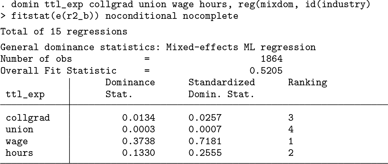
The results of this model showed that, like its effects in separating occupational categories, between-industry differences in wage also explained the most variance in between-industry differences in ttl_exp. In contrast with most models to this point, between-industry differences in the usually unimportant hours rose to second place in this model, associated with around 25% of the total between-industry variance explained in ttl_exp. Thus, differences between industries on the total experience of respondents were most strongly associated with differences between those industries on wages and hours.

5 PE-based DA analysis: domme

5.1 Command structure

domme is an extension of domin yet is far more flexible in that it can be used with sem, gsem, and any other command accepting the constraints() option. As such, the focus on domme is on creating constraints on the model that mimic the process of including versus excluding of IVs that occurs in domin.

Syntax

The command syntax is

domme [ ( eqname ₁ = parmnamelist ₁ ) … ( eqname_N = parmnamelist_N ) ][ if ] [ in ]

weight [, reg( full_estimation_command) fitstat( returned_scalar | built_in_options) [ options ]

eqname can be any equation name from that of a depvar to an implied equation such as inflate() in zip or zinb models. parmnamelists can include any varname including factor and time-series prefixed variables. Note that the function of domme‘s parenthetical statements are to produce constraints, and normal varlist expansions will not be applied. domme accepts any weights that can be used in the command entered in the reg() option.

The syntax of domme in the eqname_x = parmnamelist_x statements always creates parameter constraints of the form b[eqname:parmname] = 0, and the names submitted to it are created as such from what is typed. Thus, it is incumbent on the user to supply domme with the appropriate eqnames and parmnames for the model represented in the reg() option.

Options

reg( full_estimation_command ) refers domme to a command that accepts the option constraints(), that uses ml to estimate parameters, and that can produce the scalar in the fitstat() option. As with domin, the entry in reg() can be any official command developed by StataCorp, any community-contributed command in the SSC Archive, or any user-generated command on his or her machine. The command in reg() must accept the constraints() option. Options to the command in reg() may be passed using the ropts() option described below.

The full_estimation_command is the full estimation command, not including options following the comma, as would be submitted to Stata.

The reg() option has no default, and the user is required to provide a valid statistical model. Thus, reg() is required.

fitstat( returned_scalar | built_in_options ) refers domme to a scalar-valued model-fit summary statistic used to compute all dominance statistics. The scalar in fitstat() can be any r-class, e-class, or other scalar produced by the estimation command in reg().

In addition to fit statistics produced by the estimation command in reg(), domme also allows several built-in model fit statistics to be computed using the model log likelihood and degrees of freedom. Four fit statistics are available using the built-in options for domme. These options are the McFadden pseudo-R ² (mcf), the Estrella pseudo-R ² (est), the Akaike information criterion (aic), and the Bayesian information criterion (bic).

To instruct domme to compute a built-in fit statistic, supply the fitstat() option with an empty e-class scalar (that is, e()), and provide the three-character code for the desired fit statistic. The command in reg() must return the e(ll) value for the mcf options, must return the e(ll) and e(rank) scalars for the est and aic options, and must return the e(ll), e(rank), and e(N) scalars for the bic option. For example, to ask domme to compute McFadden’s pseudo-R ² as a fit statistic, type fitstat(e(), mcf).

Note that domme has no default, and the user is required to provide a valid fit statistic. Thus, fitstat() is required.

ropts( command_options ) includes any options that the user wants to submit to the command in the reg() option. All additional options to the command in reg() must be submitted in this option and not in the reg() option as is the case with domin.

noconditional suppresses the computation and display of conditional dominance statistics and suppresses the “strongest dominance designations” list.

nocomplete suppresses the computation of complete dominance designations and suppresses the “strongest dominance designations” list.

sets([( eqname₁_set₁ = parmnamelist₁_set₁ ) …( eqname_r_set₁ = parmnamelist_r_set₁ )] …[( eqname₁_set_N = parmnamelist₁_set_N ) …( eqname_r_set_N = parmnamelist_r_set_N )]) binds together PEs as an inseparable set in the DA. Hence, all PEs in a set will always appear together in a model and are treated as a single PE. Note that the sets of parameters must be included in brackets (that is, [ ]).

For example, consider the model glm price mpg turn trunk foreign. To produce two sets of parameters, one that includes mpg and turn as well as a second that includes trunk and foreign, type sets([(price = mpg turn)] [(price = trunk foreign)]).

This sets() statement refers to single equations within a model. A single set can include parameters from multiple equations—in fact, doing so is how IV dominance statistics can be computed in domme.

all(( eqname_all ₁ = parmnamelist_all ₁ ) … ( eqname_all_N = parmnamelist_all_N ) binds together a set of PEs to be included in all the combinations of models in the DA. Thus, all PEs included in the all() option are effectively used as covariates that are to be included in the model fit metric but for which dominance statistics will not be computed. The magnitude of the overall fit statistic associated with the set of PEs in the all() option is subtracted from the dominance statistics for all IVs and reported separately in the results. Note that the syntax to create the parmnamelists is identical to the standard domme syntax.

reverse reverses the interpretation of all dominance statistics in the e(ranking) vector and e(cptdom) matrix and fixes the computation of the e(std) vector and the “strongest dominance designations” list. domme assumes by default that higher values on overall fit statistics constitute better fit because DA has historically been based on the explained-variance R ² metric. However, DA can be applied to any model fit statistic (see Azen, Budescu, and Reiser [2001] for other examples). reverse is then useful for the interpretation of dominance statistics based on overall model fit statistics that decrease with better fit (for example, the built-in AIC, BIC statistics).

Stored results

domme stores the following in e():

Remarks

A common error is submitting b[eqname:parmname] combinations to domme that do not exist in the model. Note that submitting PE names to domme that do not exist in the model does not result in an error; domme will run despite having been given an invalid constraint but will result in unexpected effects in DA statistics. To avoid such errors, I recommend running the command in the reg() option beforehand and observing the format of the resulting e(b) matrix’s full column names to ensure the right eqname and parmnames are used.

Another important consideration is that any PEs that are not in the initial syntax’s parmnamelists, in the sets() option, or in the all() option will be considered a part of the model’s constant value and will be used as a part of the baseline log likelihoods in any built-in model fit statistic that is computed that uses it (that is, mcf and est options of fitstat(e(),…)). When using the built-in options, consider which PEs are and are not included as a part of the DA because this affects how the baseline log likelihood is computed for the McFadden and Estrella R ² metrics.

5.2 domme examples

Extending DA to multiple-equation models and PEs

As noted above, domme is an extension of the domin command and can be applied in such a way as to reproduce domin‘s results for certain commands. For example, the original mlogit, IV-based DA example above was reproducible using gsem ⁸ with sets() that group together all the PEs associated with an IV.

One results-reporting difference domme has from domin is that eqnames are reported in the results to separate PEs more easily from one another. In the above model, there were only PE sets. Thus, all results were summarized in the set equation (because sets can contain multiple eqnames).

Turning to the results in the above domme command, we find that the DA statistics from the original four-IV domin command were reproduced exactly because they were conceptually identical. In both cases, the PEs associated with each IV were either estimated or omitted from the modeling—what differs was how both methods accomplish omitting PEs or IVs. In domin, IVs were omitted from the indepvars list. In domme, PEs associated with each IV were constrained to be 0, which effectively removed them.

Whereas domme can replicate many results obtained from domin, domme extends into new analyses because any PE in a model can potentially have a dominance statistic. For example, consider a DA where the above mlogit is expanded from an IV focus to a PE focus. In this case, a PE focus would subdivide model fit contribution by PE. An example of such an analysis is outlined below.

There are several points worth noting about this PE-based DA as compared with the mlogit regression results as well as the IV-based DA. To begin, the PE-based DA bridged the gap between the original regression model and the IV-based results in that it showed more clearly how IVs and their coefficients translate into model fit across prediction equations. To illustrate, consider both wage and collgrad‘s results. The original regression results showed that collgrad had the largest single effect in separating managerial or professional from sales occupations with wage‘s effects in both prediction equations being much smaller. The PE-based DA helped to put each coefficient in the regression in context because wage‘s much higher variability was taken into account for the PE-based DA. In fact, the PE-based DA showed that the strongest PE was wage in separating managerial or professional from other occupations and that the effect of collgrad in separating managerial or professional from sales occupations was ranked second. Such information would be difficult to glean from the regression results alone.

The PE-based DA also added useful detail to the results from the IV-based DA. In this case, the IV-based DA determined that wage was on average the strongest IV yet, and the PE-based DA showed its two individual PEs are not ranked as the top two. Rather, wage had the first-ranked PE as noted above along with the third-ranked PE separating managerial or professional from sales occupations. Together, wage‘s PEs combined to make wage the most important IV, but, when separated, collgrad‘s managerial or professional from sales occupations PE was also determined to be quite strong and actually outranked one of wage‘s PEs by a fair margin. This information would not be ascertainable from the IV-based DA results alone.

Note that PE-based DA results do not necessarily sum to exactly their IV-based results. For example, the sum of the PE-based DA results for wage was 0.0416+0.0122 = 0.0538, very similar but not identical to the IV-based value of 0.0537. This is because the PE-based results account for correlations between prediction equations within the same IV that are ignored when the PEs are grouped. Consequently, PE-based results will not cleanly decompose into components of their IV-based results but will generally be similar.

More extensive multiple-equation model

In a final example, the original mlogit was extended to a multiple-phase prediction model where the IVs in the original model were themselves predicted by another IV. In this case, the respondent’s total years of work experience (ttl_exp, as in the mixdom example) increased the likelihood of a respondent being a college graduate and a union member. Total work experience also increased respondents’ hours worked and their pay. These experience effects were built into the system of relationships already known about occupation categories. Of interest for this extension of the models above was discerning which prediction paths appeared to have the most impact overall in understanding occupational sorting. That is, how predictable were the IVs using ttl_exp, and, subsequently, how well did the IVs predict occ_cat?

The domme results suggested that the path predicting through wages appeared to have the most impact in the context of the model. This is because wage, as a dependent and independent variable, was incorporated into the top two PEs and accounted for 53.73% of the R ² value when summed.

collgrad obtained the fourth-ranked PE for its effect in predicting occupation sorting but had a much weaker relationship with work experience; hence, collgrad predicted well but was not as predictable. By contrast, hours obtained the third-ranked PE in being predicted by work experience but a much weaker effect in predicting occupational sorting; it was predictable but did not predict as well. In comparing both, we found hours showed a stronger total impact than collgrad. hours accounted for 22.08% of the R ² value when summed, whereas collgrad accounted for 16.41% of the R ² value. Thus, on the whole, the model explained more with hours than collgrad.

The example above illustrates that the domme program can obtain importance comparisons for a wide variety of models, many of which would be otherwise difficult to dominance-analyze. domme can collect dominance statistics across prediction equations with multiple distribution types and IV variances. For example, domme permitted comparisons across PEs like b[2.occ_cat:union], a binary variable predicting a betweencategory relative rate in a multinomial logit and b[hours:ttl_exp], a continuous variable predicting another continuous variable in a linear regression. In each case, dominance statistic values were based on change in the model log likelihood. The shared underlying metric of the model log likelihood is a standardized metric that is comparable across PEs using dominance statistics despite their difference in distribution form. Making such comparisons across prediction equations is difficult to do outside the DA framework.

Note that the shared metric of the log likelihood had another implication for the domme model presented above. As can be seen, the McFadden pseudo-R ² was 0.0179, a fairly low value, especially compared with the mlogit models considered previously. This is because gsem had five different dependent variables that contributed to the log likelihood: occ_cat, wage, hours, collgrad, and union. Explaining information about the model was balanced across all five dependent variables and not just occ_cat as before. As the lower value suggests, the four newly introduced dependent variables were not, on the whole, explained well given the model.

Now that multiple examples of IV- and PE-based DA have been outlined, I turn to discuss an important consideration for DA: computation time to collect the entire ensemble of fit statistics required to compute dominance statistics.

6 Computational considerations

Because DA must estimate all possible subsets of IVs or PEs estimated or omitted from the base model, it is a computationally intensive methodology. Indeed, increasing the number of IVs or PEs in the DA results in a geometric increase in the number of models run. Most modern computers can probably easily handle IV or PE counts up to around 15 (that is, 32,767 models) with no problem. Beyond 15, the hardware on the user’s machine may begin to make a difference in terms of run time and likelihood of the method successfully completing. Implementing DA at a larger scale may require the user to choose a different strategy to obtain dominance statistics.

The simplest method to scale up DA is to use the epsilon option. This option produces an approximation to the general dominance statistics using singular value decomposition (see Johnson [2000]) and requires running only a single model. However, the epsilon option is limited in that it is only implemented for domin, cannot produce conditional or complete dominance statistics, cannot accommodate sets() or all(), and can be run only for regress, mvreg, and glm models. The epsilon approach is implemented such that each model it can accommodate has a unique method built into domin. Future work may seek to extend the number of built-in models or generalize the approach such that each model being run does not need its own unique method. Currently, epsilon is the best method to use to expedite DA when the user’s statistical model can be accommodated.

Another alternative is to utilize multiprocessing on a single computer or network of computers to expedite run time. DA is an approach that fits many independent models (that is, each model run in the ensemble needs no input from another model in the ensemble) and thus can be parallelized such that different processors compute different models simultaneously. In fact, because the models share no information, the DA method is what is known as an “embarrassingly parallel” task that can be parallelized without any losses in computation efficiency. Currently, domin and domme are not parallelized, and each model is run serially: one after another until complete. Stata has a few methods that could be implemented to parallelize the fitting of all possible combinations of models necessary for DA. For example, the parallel (Vega Yon and Quistorff 2019) module described in a recent Stata Journal article describes how to divide up computationally intensive tasks like bootstrap sampling to parallelize them on a single machine that could be applied in DA. Similar approaches are taken with the SSC modules qsub(Sayers 2017) and multishell(Ditzen 2018). Additionally, Stata version 16’s integration with Python could allow for the adaptation of its flexible multiprocessing module which can also call multiple instances of Stata and features sophisticated subroutines for controlling the multiple processes used to estimate all possible combinations. One constraint with any multiprocessing approach will be in memory requirements to implement. Because Stata holds the data on which models are run in memory, each instance of Stata called (that is, each parallel process) will require more memory. This method may thus be feasible only with computers with both multiple processors and high amounts of random access memory available. Also note that this method is a potential future direction and is not currently implemented for domin and domme.

A final alternative is to reduce computational burden through a different approximation approach than epsilon. One potentially fruitful alternative approach would use model subsampling. That is, finding a subset of the entire ensemble of 2 ^p−1 such that when dominance statistics are computed using that subset, the dominance statistics generated are an unbiased estimate of the statistics that would be produced by the all-possible-subsets approach. Ultimately, this last subsampling is likely to be the most practical way forward because it can reproduce the information expected from a full DA, can be tuned to ensure the statistics obtained are not unduly biased, and yet dramatically reduce the total number of models fit. As with the multiprocessing suggestion, this method is a potential future direction and is not currently implemented for domin and domme.⁹

7 Discussion

Relative importance methods like DA have a long history in statistics as well as research methodology and are useful for presentation of statistical model results. DA is useful in that it supplements the information offered by regression coefficients with the impact that IVs and PEs have on explaining the dependent variables in the model (for example, Tonidandel and LeBreton [2011]). Moreover, the DA methods implemented here permit comparisons of PEs that have, heretofore, been difficult to compare directly, such as Poisson with logit coefficients across prediction equations in a zero-inflated Poisson (zip) regression.

Historically, a barrier to using many relative importance methodologies, such as DA, has been the unavailability of easy-to-use software to implement the computations. The two commands discussed in this work provide a framework based on Stata’s structured syntax and can accommodate a broad cross-section of potential regression models. This is a key advantage of domin and domme because published work on DA has been extended to only a few models, including regress, logit, ologit, mlogit, mvreg, and mixed. With these commands, a user can apply DA to each of these models but also to any other official, community-contributed, or user-generated statistical models fittable in Stata that can fit into the same syntax. For example, domin can easily fit poisson, streg, tobit, fracreg, and xtreg as well as others (for example, glm, qreg) with a wrapper program in a style similar to mvdom or mixdom.¹⁰ domme can apply to many more models, including sureg, gsem, zip, and betareg, as well as many panel-data models (for example, xtlogit) and choice models (for example, cmclogit). Currently, domme does not work with multilevel mixed-effects models fit through commands such as melogit but can be used through the methods offered to fit such models in gsem.

In closing, I have outlined how domin and domme can provide additional information about statistical models fit in Stata and allow for comparisons between effects that previously would have been difficult to compare. The flexibility of these programs requires good judgment in application, and I remind readers that the comparisons made between IVs and PEs must be conceptually reasonable and that model-selection processes must precede the DA. When one follows standard statistical practice, DA can be helpful and add value for translating model results into relative explanatory usefulness for IVs and PEs.

8 Programs and supplemental materials

Supplemental Material, sj-zip-1-stj-10.1177_1536867X211025837 - Determining relative importance in Stata using dominance analysis: domin and domme

Supplemental Material, sj-zip-1-stj-10.1177_1536867X211025837 for Determining relative importance in Stata using dominance analysis: domin and domme by Joseph N. Luchman in The Stata Journal

Footnotes

8 Programs and supplemental materials

To install a snapshot of the corresponding software files as they existed at the time of publication of this article, type

Notes

References

Azen

Budescu

D. V.

2006. Comparing predictors in multivariate regression models: An extension of dominance analysis. Journal of Educational and Behavioral Statistics 31: 157–180. https://doi.org/10.3102/10769986031002157.

Azen

Budescu

D. V.

Reiser

2001. Criticality of predictors in multiple regression. British Journal of Mathematical and Statistical Psychology 54: 201–225. https://doi.org/10.1348/000711001159483.

Budescu

D. V.

1993. Dominance analysis: A new approach to the problem of relative importance of predictors in multiple regression. Psychological Bulletin 114: 542–551. https://doi.org/10.1037/0033-2909.114.3.542.

Budescu

D. V.

Azen

2004. Beyond global measures of relative importance: Some insights from dominance analysis. Organizational Research Methods 7: 341–350. https://doi.org/10.1177/1094428104267049.

Ditzen

2018. multishell: Stata module to allot do files and variations of loops across parallel instances of Windows Stata and computers efficiently. Statistical Software Components S458512, Department of Economics, Boston College. https://EconPapers.repec.org/RePEc:boc:bocode:s458512.

Grömping

2007. Estimators of relative importance in linear regression based on variance decomposition. American Statistician 61: 139–147. https://doi.org/10.1198/000313007X188252.

Johnson

J. W.

2000. A heuristic method for estimating the relative weight of predictor variables in multiple regression. Multivariate Behavioral Research 35: 1–19. https://doi.org/10.1207/S15327906MBR3501_1.

Johnson

J. W.

LeBreton

J. M.

2004. History and use of relative importance indices in organizational research. Organizational Research Methods 7: 238–257. https://doi.org/10.1177/1094428104266510.

Juarez

F. C

. 2012. shapley2: Stata module to compute additive decomposition of estimation statistics by regressors or groups of regressors. Statistical Software Components S457543, Department of Economics, Boston College. https://EconPapers.repec.org/RePEc:boc:bocode:s457543.

10.

Kolenikov

2000. shapley: Stata module to perform additive decomposition of sample statistic. Statistical Software Components S411401, Department of Economics, Boston College. https://EconPapers.repec.org/RePEc:boc:bocode:s411401.

11.

LeBreton

J. M.

Ployhart

R. E.

Ladd

R. T.

2004. A Monte Carlo comparison of relative importance methodologies. Organizational Research Methods 7: 258–282. https://doi.org/10.1177/1094428104266017.

12.

LeBreton

J. M.

Tonidandel

2008. Multivariate relative importance: Extending relative weight analysis to multivariate criterion spaces. Journal of Applied Psychology 93: 329–345. https://doi.org/10.1037/0021-9010.93.2.329.

13.

Luchman

J. N.

2014. Relative importance analysis with multicategory dependent variables: An extension and review of best practices. Organizational Research Methods 17: 452–471. https://doi.org/10.1177/1094428114544509.

14.

Luchman

J. N.

Klein

Cox

N. J.

2006. tuples: Stata module for selecting all possible tuples from a list. Statistical Software Components S456797, Department of Economics, Boston College. https://EconPapers.repec.org/RePEc:boc:bocode:s456797.

15.

Luchman

J. N.

Lei

Kaplan

S. A.

2020. Relative importance analysis with multivariate models: Shifting the focus from independent variables to parameter estimates. Journal of Applied Structural Equation Modeling 4: 1–20. https://doi.org/10.47263/JASEM.4(2)02.

16.

Luo

Azen

2013. Determining predictor importance in hierarchical linear models using dominance analysis. Journal of Educational and Behavioral Statistics 38: 3–31. https://doi.org/10.3102/1076998612458319.

17.

Sayers

2017. qsub: Stata module to emulate a cluster environment using your desktop PC. Statistical Software Components S458366, Department of Economics, Boston College. https://EconPapers.repec.org/RePEc:boc:bocode:s458366.

18.

Thomas

D. R.

Zumbo

B. D.

Kwan

Schweitzer

2014. On Johnson’s (2000) relative weights method for assessing variable importance: A reanalysis. Multivariate Behavioral Research 49: 329–338. https://doi.org/10.1080/00273171.2014.905766.

19.

Tonidandel

LeBreton

J. M.

2010. Determining the relative importance of predictors in logistic regression: An extension of relative weight analysis. Organizational Research Methods 13: 767–781. https://doi.org/10.1177/1094428109341993.

20.

Tonidandel

LeBreton

J. M.

2011. Relative importance analysis: A useful supplement to regression analysis. Journal of Business and Psychology 26: 1–9. https://doi.org/10.1007/s10869-010-9204-3.

21.

Vega Yon

G. G.

Quistorff

2019. parallel: A command for parallel computing. Stata Journal 19: 667–684. https:///doi.org/10.1177/1536867X19874242.

Supplementary Material

Please find the following supplemental material available below.

For Open Access articles published under a Creative Commons License, all supplemental material carries the same license as the article it is associated with.

For non-Open Access articles published, all supplemental material carries a non-exclusive license, and permission requests for re-use of supplemental material or any part of supplemental material shall be sent directly to the copyright owner as specified in the copyright notice associated with the article.

0.00 MB