Sage Journals: Discover world-class research

Abstract

In this article, we describe the mlcar command, which implements a maximum likelihood method to simultaneously estimate the regression coefficients of a two-regime endogenous switching model and the coefficient measuring the correlation of outcomes between the two regimes. This coefficient, known as the “across-regime” correlation parameter, is generally unidentified in the traditional estimation procedures.

Keywords

st0642 mlcar mlcartestn Roy model endogenous switching maximum likelihood across-regime correlation

1 Introduction

The two-regime switching regression models have been widely used in applied economic analysis, such as in the estimation of the earnings equations for unionized and nonunionized workers or in the estimation of wage equations of subjects employed in the private sector and in the public sector (Lee 1978; Lee and Trost 1978). Researchers have adopted several estimation methods to obtain estimates of the coefficients of the outcome equations in both regimes. The model is usually extended, and a further selection equation is included. Within this framework, maximum likelihood (ML) methods (Poirier and Ruud 1981; Maddala 1983) and two-stage procedures (Heckman 1976, 1990; Lee 1978) provided estimated coefficients of the outcome equations and of the selection equation, including variances of the error terms and covariances between the errors of the outcome equations and the selection equation.¹ In such models, the selection equation allows one to identify the choice of the regime (the decision of the agent of belonging to regime 1 or to regime 2) supporting the two outcome equations. The estimation of the outcome equations in both regimes accounts for the endogenous effect of the selection by introducing, in the respective regressors set, a correction term obtained by the “generalized residuals” of the selection equation, estimated at a first stage.

In general, the two-stage method was recognized as consistent and computationally feasible. The ML approach also considers the same three-equation set, simultaneously estimating all parameters.

However, these methods did not provide the estimation of the parameter measuring the correlation between the error terms of the two outcome equations, the so-called across-regime correlation (or covariance). The reason is that this parameter is not empirically identifiable because of the selection rule specifying a two-regime switching model, in which the dependent variable referred to an observation cannot be jointly observed in both regimes.

Despite the difficulty in identification, some “knowledge” about this parameter was considered relevant in terms of interpretation of the agent’s behavior in an endogenous switching model (see Heckman and Honoré [1990] and Vijverberg [1993]). The across-regime correlation measures the correlation in unobserved productivity (ability) of the subject in both regimes (or sectors). The traditional estimation methods allow estimating the cross-correlation parameter only “indirectly”, based on the estimate of coefficients and variances, and applying the relationships among the errors’ second-order moments as in Maddala (1983, 223–228) and in French and Taber (2010).

Differently from these approaches, which provide an “indirect” estimation of the across-regime correlation parameter, Calzolari and Di Pino (2017) suggested that identification and direct ML estimation of the across-regime correlation parameter are possible if the model specification is closer to the traditional Roy model rather than its more widely used generalized versions. The model is specified as “two equation”, implying a sort of “rational” behavior of the agent, who simply chooses the regime with the higher outcome. For each individual, the contribution to the likelihood is given by the probability density of the observed (larger) outcome and by the (conditional) probability that the alternative (censored) outcome has a smaller value.

This approach allows us to obtain a reliable simultaneous point estimation of both the outcome equations without introducing a further selection equation explaining the choice of the subject, such as in the specification of the “generalized” Roy model (for example, Carneiro, Hansen, and Heckman [2003]). This allows us to obtain more efficient estimates than those provided applying two-stage estimation methods.²

In this article, we describe the mlcar command, which implements the two-equation ML method of Calzolari and Di Pino (2017) to estimate simultaneously the coefficients of an (endogenous switching) two-equation model including the across-regime correlation coefficient. This full-information approach relies on the assumption of joint normality of the error terms of each of the two outcome equations in the respective regime.

In the next section, we briefly discuss the properties of the across-regime correlation coefficient and its relevance for economic analysis. In section 3, we provide a brief description of the methodology and model specification.

Because our full-information approach relies on the assumption of normality of the error terms in each regime, we also provide a postestimation command to verify the hypothesis of normality of the error terms in both regimes (mlcartestn). This testing procedure is an extension to the two-regime endogenous switching models of the conditional moment (CM) test, which verifies the normality assumption in the censored regression model (tobit; see, for example, Newey [1985]; Tauchen [1985]; Skeels and Vella [1999]). We report a brief description of this procedure in section 3.1.

In section 4, we describe the mlcar command and its options followed by general examples of application. In section 5, we report the results of some empirical applications of the mlcar command.

To provide a comparison with the mlcar results, in the appendix, we consider the procedure that should be applied for the indirect estimation of the cross-correlation coefficient if the endogenous switching model is estimated in one of the traditional ways. Appendix A briefly describes how to obtain the indirect estimate of the across-regime correlation parameter via the two-stage Heckman procedure, and in appendix B, we consider the same empirical applications of section 5 and report the indirect estimation of this parameter. Finally, in appendix C, we report the results of several Monte Carlo experiments, checking the performance of the CM test statistics by simulating data with different distributions of the error terms.

2 Relevance and empirical content of the across-regime correlation coefficient

In many cases, the two-regime switching models extend the Roy model of self-selection to include the decision rule adopted for selecting into different regimes. For example, the two-regime wage’s model of self-selection aims to explain the workers’ occupational choice and its consequences for the distribution of earnings when individuals differ in their endowments of specific skills (see Heckman and Honoré [1990]; Vijverberg [1993]). In doing this, one should obtain information about the joint distribution of the potential (counterfactual) outcomes. A relevant parameter of such a distribution is the across-correlation coefficient, ρ ₁₂.³

Heckman and Honoré (1990) proved that the identification of the joint distribution of potential outcomes is essential to the empirical content of this model. As shown by these authors, if the ρ ₁₂ coefficient is identified, one can, by adopting a two-regime specification as in a Roy model, estimate the population distribution of potential outcomes knowing only the outcomes of subjects observed into one of the two regimes.

The sign of the across-regime correlation, in particular, allows us to know more in detail what criterion the agents follow to select the regime. Considering a wage model in a public or private sector choice, for example, a positive sign of ρ ₁₂ signals that the agents, supported by their own skills, manage to gain a higher-than-average level of outcome in both regimes. Thus, one of the two sectors (public sector) absorbs most of the above-average productive workers.

At the opposite, a negative sign of ρ ₁₂ means that the agent has different skills in each regime, and he or she chooses the regime in which he or she is more productive. In this case, the workers are absorbed by the sector in which they gain a comparative advantage in terms of productivity. This condition generally increases the segmentation of the labor market.

An example on the use of ρ ₁₂ to obtain information about the skills of the agents is provided by Calzolari and Di Pino (2017), who estimated the time devoted to domestic work by employed and unemployed women in Italy. In this case, a positive sign of ρ ₁₂ indicated that common latent factors positively influence the domestic work supply of women in both regimes. This result led to the conclusion that employed and unemployed women do not have different skills regarding their commitment in domestic work.

Some studies showed that a knowledge of the ρ ₁₂ coefficient supports methods for obtaining the predictive distributions of outcomes and, consequently, an estimation of the treatment parameters (average treatment effect, average treatment effect on the treated) measuring outcome gains from program participation. Poirier and Tobias (2003), in particular, showed how the entire distribution associated with these gains can be obtained in certain situations if the ρ ₁₂ coefficient is, at least in part, identified.

Along this line, Fan and Wu (2010) provide sharp bounds to obtain a partial identification of the correlation coefficient of the potential outcomes, their joint distribution, and the distribution of treatment effects.

The aforementioned studies on the use of two-regime switching models adopt partial information on the ρ ₁₂ coefficient to derive predictive distributions. Instead, an important result achieved by applying the estimator implemented by the mlcar procedure consists in obtaining a direct point estimation of the ρ ₁₂ parameter, supported by the typical inferential properties of the ML estimators.

3 Methodological issues

Calzolari and Di Pino (2017) specified an endogenous switching model with two regression equations whose dependent variables (outcomes) are mutually exclusive in a cross-sectional framework and where selection is simply based on the choice of the larger outcome.

\begin{array}{l} y_{1 i} = x_{1 i}^{'} β_{1} + u_{1 i} if observed in regime 1; otherwise latent \\ y_{2 i} = x_{2 i}^{'} β_{2} + u_{2 i} if observed inregime 2; otherwise latent \end{array}

The agent is assumed to behave rationally; thus, if y ₁ _i > y ₂ _i , then y ₁ _i is observed and y ₂ _i is latent; otherwise, y ₂ _i is observed and y ₁ _i is latent.

A relevant characteristic of this model is that the two dependent variables, y ₁ _i and y ₂ _i , are explicitly factors in the choice of the regime. For each individual, y ₁ _i − y ₂ _i represents the net gain (or net loss) from the choice between two options.

The error terms u ₁ _i and u ₂ _i , given by $u_{1 i} = y_{1 i} - x_{1 i}^{'} β_{1}$ and $u_{2 i} = y_{2 i} - x_{2 i}^{'} β_{2}$ , are assumed to be normally distributed with zero mean and variances σ ₁ ² and σ ₂ ². Identification and estimation of the across-regime covariance, σ ₁₂, becomes possible by considering (as in a tobit model) the probability density of the observed outcome, multiplied by the conditional probability that the other outcome (latent) is smaller than the observed. More in detail, the censoring rule in the model implies that

\begin{array}{l} y_{1 i} observed \Rightarrow y_{2 i} < y_{1 i} \Rightarrow x_{2 i}^{'} β_{2} + u_{2 i} < y_{1 i} \\ y_{2 i} observed \Rightarrow y_{1 i} \leq y_{2 i} \Rightarrow x_{1 i}^{'} β_{1} + u_{1 i} \leq y_{2 i} \end{array}

Hence,

\begin{array}{l} ϕ (y_{1 i}) P (y_{2 i} < y_{1 i}) = ϕ (u_{1 i}) P (u_{2 i} < y_{1 i} - x_{2 i}^{'} β_{2} y_{1 i} observed) \\ ϕ (y_{2 i}) P (y_{1 i} \leq y_{2 i}) = ϕ (u_{2 i}) P (u_{1 i} \leq y_{2 i} - x_{1 i}^{'} β_{1} y_{2 i} observed) \end{array}

where φ(·) is a normal probability density function.

We consider also the CMs of the error terms; namely, $E (u_{1 i} | u_{2 i}) = (σ_{12} / σ_{2}^{2}) u_{2 i} = (σ_{12} / σ_{2}^{2}) (y_{2 i} - x_{2 i}^{'} β_{2})$ and $Var (u_{1 i} | u_{2 i}) = σ_{1}^{2} - (σ_{12}^{2} / σ_{2}^{2})$ are, respectively, the conditional mean and variance of u ₁ _i given u ₂ _i . Analogously, $E (u_{2 i} | u_{1 i}) = (σ_{12} / σ_{1}^{2}) u_{1 i} = (σ_{12} / σ_{1}^{2}) (y_{1 i} - x_{1 i}^{'} β_{1}$ and $Var (u_{2 i} | u_{1 i}) = σ_{2}^{2} - (σ_{12}^{2} / σ_{1}^{2})$ are, respectively, the conditional mean and variance of u ₂ _i given u ₁ _i . Hence, σ ₁₂ is the covariance between the error terms of both regimes, known as the across-regime covariance.

Therefore, in (1) we have the probability that an agent does not belong to regime 2, under the condition that he or she chooses regime 1:

P (u_{2 i} \leq y_{1 i} - x_{2 i}^{'} β_{2} y_{1 i} observed) = Φ {\frac{(y_{1 i} - x_{2 i}^{'} β_{2}) - \frac{σ_{12}}{σ_{1}^{2}} (y_{1 i} - x_{1 i}^{'} β_{1})}{\sqrt{σ_{2}^{2} - σ_{12}^{2} / σ_{1}^{2}}}}

Analogously, in (2) we have the probability that an agent does not belong to regime 1, under the condition that he or she chooses regime 2:

P (u_{1 i} \leq y_{2 i} - x_{1 i}^{'} β_{1} y_{2 i} observed) = Φ {\frac{(y_{2 i} - x_{1 i}^{'} β_{1}) - \frac{σ_{12}}{σ_{2}^{2}} (y_{2 i} - x_{2 i}^{'} β_{2})}{\sqrt{σ_{1}^{2} - σ_{12}^{2} / σ_{2}^{2}}}}

Φ(·) is the standard normal cumulative distribution function used to specify, in both (1) and (2), the contribution to the likelihood of censoring, respectively, y ₂ _i and y ₁ _i .

Therefore, given the conditional probabilities (1) and (2), we finally obtain the following contribution of the ith observation to the log likelihood,

\begin{array}{l} \ln L {(θ)}_{i} = R_{i} [- \frac{{(y_{1 i} - x_{1 i} β_{1})}^{2}}{2 σ_{1}^{2}} - \frac{1}{2} \ln σ_{1}^{2} + \ln Φ {\frac{(y_{1 i} - x_{2 i}^{'} β_{2}) - \frac{σ_{12}}{σ_{1}^{2}} (y_{1 i} - x_{1 i}^{'} β_{1})}{\sqrt{σ_{2}^{2} - σ_{12}^{2} / σ_{1}^{2}}}}] \\ + (1 - R_{i}) [- \frac{{(y_{2 i} - x_{2 i}^{'} β_{2})}^{2}}{2 σ_{2}^{2}} - \frac{1}{2} \ln σ_{2}^{2} + \ln Φ {\frac{(y_{2 i} - x_{1 i}^{'} β_{1}) - \frac{σ_{12}}{σ_{2}^{2}} (y_{2 i} - x_{2 i}^{'} β_{2})}{\sqrt{σ_{1}^{2} - σ_{12}^{2} / σ_{2}^{2}}}}] \end{array}

with $θ = {(β_{1}^{'}, β_{2}^{'}, σ_{1}^{2}, σ_{2}^{2}, σ_{12})}^{'}$ , while R_i is a dummy-indicator variable equal to 1 if y ₁ _i is observed (regime 1) and equal to 0 if y ₂ _i is observed (regime 2). Applying this two-equation ML procedure, we can directly estimate the parameter σ ₁₂ (or ρ ₁₂) under the assumption of endogenous selection.

3.1 A CM test of normality for a two-regime switching model

The ML estimator critically relies on the assumption of normality of the error terms of both equations. As a complement to the estimation procedure, we implement a CM test to verify the normality assumption. The proposed test procedure extends, to the two-equation case, the CM test available in the literature to verify the normality assumption in the context of the tobit model (for example, Skeels and Vella [1999]). In particular, the test is based on the comparison of the third and fourth moments of u ₁ _i and u ₂ _i with the theoretical values implied under the assumption of normally distributed error terms. Absent censoring, we could write

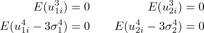
\begin{matrix} E (u_{1 i}^{3}) & = 0 & E (u_{2 i}^{3}) & = 0 \\ E (u_{1 i}^{4} - 3 σ_{1}^{4}) & = 0 & E (u_{2 i}^{4} - 3 σ_{2}^{4}) & = 0 \end{matrix}

However, these equalities cannot be satisfied on the “observed” part of each regime, because of censoring.

The CM test is built by considering the following observed residuals:

\begin{array}{l} v_{3 i} = R_{i} {u_{1 i}^{3} - E (u_{1 i}^{3} y_{1 i} observed)} + (1 - R_{i}) {u_{2 i}^{3} - E (u_{2 i}^{3} y_{2 i} observed)} \\ v_{4 i} = R_{i} {u_{1 i}^{4} - E (u_{1 i}^{4} y_{1 i} observed)} + (1 - R_{i}) {u_{2 i}^{4} - E (u_{2 i}^{4} y_{2 i} observed)} \end{array}

The moment conditions that we exploit to verify the normality assumption can therefore be written as

\begin{array}{l} E (v_{3 i}) = 0 \\ E (v_{4 i}) = 0 \end{array}

with v ₃ _i and v ₄ _i including powers of the observed residuals in regime 1 and regime 2 as defined before.

For observations in regime 1, we can write

{\hat{u}}_{1 i}^{3} = {(y_{1 i} - x_{1 i}^{'} {\hat{β}}_{1})}^{3} and {\hat{u}}_{1 i}^{4} = {(y_{1 i} - x_{1 i}^{'} {\hat{β}}_{1})}^{4}

Analogous formulas hold for observations in regime 2:

{\hat{u}}_{2 i}^{3} = {(y_{2 i} - x_{2 i}^{'} {\hat{β}}_{2})}^{3} and {\hat{u}}_{2 i}^{4} = {(y_{2 i} - x_{2 i}^{'} {\hat{β}}_{2})}^{4}

To perform the computations related to the testing procedure, we also need to evaluate the following CMs:

\begin{matrix} E (u_{1 i}^{3} | y_{1 i} observed) & E (u_{2 i}^{3} | y_{2 i} observed) \\ E (u_{1 i}^{4} | y_{1 i} observed) & E (u_{2 i}^{4} | y_{2 i} observed) \end{matrix}

Focus on the computation related to u ₁ _i ; an analogous formula applies for u ₂ _i .

Under the assumption of joint normality of u ₁ _i and u ₂ _i , we note that the difference δ_i = u ₁ _i − u ₂ _i is also normally distributed. Thus, u ₁ _i can be written as a linear function of δ_i plus an independent error term,

u_{1 i} = τ_{1} δ_{i} + ϵ_{1 i}

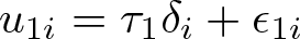
with ϵ ₁ _i normally distributed, independent of δ_i , and τ ₁ = cov(δ_i, u ₁ _i )/var(δ_i ). It holds that $E (ϵ_{1 i}) = 0, E (ϵ_{1 i}^{2}) = σ_{ϵ}^{2}, E (ϵ_{1 i}^{3}) = 0$ , and $E (ϵ_{1 i}^{4}) = 3 σ_{ϵ}^{4}$ . We therefore can write

\begin{array}{l} E (u_{1 i}^{3} | y_{1 i} observed) = E {{(τ_{1} δ_{i} + ϵ_{1 i})}^{3} | δ_{i} \leq x_{1 i}^{'} β_{1} - x_{2 i}^{'} β_{2}} \\ E (u_{1 i}^{4} | y_{1 i} observed) = E {{(τ_{1} δ_{i} + ϵ_{1 i})}^{4} | δ_{i} \leq x_{1 i}^{'} β_{1} - x_{2 i}^{'} β_{2}} \end{array}

The two expected values can be computed by exploiting the recursive formula that characterizes the moments of a truncated normal distribution (see, for example, Chesher and Irish [1987, 40]) and exploiting the independence of ϵ ₁ _i and δ_i (see also Pfaffermayr [2014]).

The computation in mlcartestn is based on the outer-product-gradient formula: consider the vector w _i , which includes the gradient of the log likelihood function (3) and the residuals,

w_{i} = (\frac{\partial \ln L_{i}}{\partial θ^{'}}, {\hat{v}}_{3 i}, {\hat{v}}_{4 i})

with $θ = {(β_{1}^{^{'}}, β_{2}^{^{'}}, σ_{2}^{1}, σ_{2}^{2}, σ_{12})}^{'}$ . Build the matrix W with rows w _i . The test is obtained as

CM = ι^{'} W {(W^{'} W)}^{- 1} W^{'} ι

with ι a column vector of ones. The test corresponds to nR ² with the uncentered coefficient of determination of the regression of ι on w _i . Computed in this form, the test is known to have small-sample problems in finite samples (for example, Drukker [2002]); it is oversized in finite samples. To address this issue, we also provide a simulated version of the CM test as in Orme (1995).

4 The mlcar command

4.1 Syntax

mlcar fits a two-equation endogenous switching model using the procedure described in Calzolari and Di Pino (2017). The dependent variable (depvar) is recorded across two regimes, as identified by the selection variable specified in the (required) option regime( varname ). The generic syntax for the command is as follows:

mlcar depvar [ if ] [ in ] [ weight [, regime( varname ) x1( varlist ) [ x2( varlist ) accuracy(0 | 1 | 2) olsinit level( # ) maximize_options ]

fweights, aweights, iweights, and pweights are allowed; see [U] 11.1.6 weight.

The dependent variable depvar is recorded across two regimes, as identified by the variable specified in the (required) option regime( varname ):

\begin{array}{l} y_{1} = depvar if varname = 1 \\ y_{2} = depvar if varname = 0 \end{array}

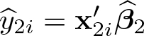
It is assumed that the individual chooses the regime with the highest outcome; that is,

\begin{array}{l} y_{2} \geq y_{1} if varname = 0 \\ y_{2} < y_{1} if varname = 1 \end{array}

The variances of the error terms of the outcome equations are $σ_{1}^{2} = s 11$ and $σ_{2}^{2} = s 22$ , and the covariance between the two error terms is σ ₁₂ = s12. The across-regime correlation can be computed as ρ ₁₂ = r12 = s12/sqrt(s11 × s22).⁴

4.2 Options

regime() identifies the variable that specifies the two regimes, one coded as 0 (y ₂ is recorded in depvar) and the other as equal to 1 (y ₁ is recorded in depvar). regime() is required.

x1( varlist ) and, optionally, x2( varlist ) specify the list of variables. When the same set of regressors $XLIST is specified in both outcome equations, these can be specified in the (required) option x1() as x($XLIST). However, the set of regressors in x1() and x2() need not be the same: a different list of variables can be specified in x1() and in x2() to be used as independent variables for the outcome equation of regime 1 and 2, respectively. x1() is required.

accuracy() defines how the gradient vector and the Hessian matrix are computed:

If accuracy(0), both gradient and Hessian are obtained in a numeric way (method(lf0) is used with the ml command).

If accuracy(1), the gradient vector is computed using the analytic formula (method(lf1) is used with the ml command; the Hessian is still computed using numeric approximation).

If accuracy(2) (the default), both gradient and Hessian are computed using the analytic formula (method(lf2) is used with the ml command).

olsinit specifies to use the ordinary least-squares estimates as initial values for the ml estimation (in this case, the starting value of r12 is set equal to 0). Alternatively, the user can specify different initial values using the option init( ml_init_args ), available with the ml command. If no initial value is specified, mlcar lets the ml command search for initial values.

level( # ) specifies the confidence level. By default, the value in macro S_level is considered. The default is level(95).

maximize_options specifies the options of the Stata command ml model; see [R] ml for details.

4.3 Postestimation

The postestimation command predict can be used after mlcar. The syntax is

predict newvar [ , xb1 xb2 pnb12 pnb21]

The following options are allowed to compute these conditional and unconditional expectations:

xb1 calculates the linear prediction in regime 1 for observations in regime 1 and in regime 2 (the default):

{\hat{y}}_{1 i} = x_{1 i}^{'} {\hat{β}}_{1}

xb2 calculates the linear prediction in regime 2 for observations in regime 2 and in regime 1:

{\hat{y}}_{2 i} = x_{2 i}^{'} {\hat{β}}_{2}

pnb12 calculates the probability of not being in regime 1, for units deciding to belong to regime 2:

Φ {\frac{(y_{2 i} - x_{1 i}^{'} {\hat{β}}_{1}) - \frac{{\hat{σ}}_{12}}{{\hat{σ}}_{2}^{2}} (y_{2 i} - x_{2 i}^{'} {\hat{β}}_{2})}{\sqrt{{\hat{σ}}_{1}^{2} - {\hat{σ}}_{12}^{2} / {\hat{σ}}_{2}^{2}}}}

pnb21 calculates the probability of not being in regime 2, for units deciding to belong to regime 1:⁵

Φ {\frac{(y_{1 i} - x_{2 i}^{'} {\hat{β}}_{2}) - \frac{{\hat{σ}}_{12}}{{\hat{σ}}_{1}^{2}} (y_{1 i} - x_{1 i}^{'} {\hat{β}}_{1})}{\sqrt{{\hat{σ}}_{2}^{2} - {\hat{σ}}_{12}^{2} / {\hat{σ}}_{1}^{2}}}}

After mlcar, mlcartestn performs the CM test for joint normality of the error terms. The default computation of the test statistics uses the outer-product-gradient form (Skeels and Vella 1999). The syntax is

mlcartestn[ , sim( # )]

sim( # ) permits one to compute the simulated version of the CM test as in Orme (1995).

5 Examples

We illustrate the use of the mlcar command with four examples. The first two datasets used are available from Wooldridge (2010) and readable within Stata (https://www.stata.com/texts/eacsap/); the third dataset is used by Hamermesh and Biddle (1994), and it can be downloaded from http://fmwww.bc.edu/ec-p/data/wooldridge/beauty.dta.

Still on page 6, three lines before the end or the page, in the expression of the conditional variance, σ ₁₂ should be squared.

At the top of page 7, after (10), the lines 2 and 3 should be written as “Analogously, the probability of a subject not belonging to regime 2 under the condition that he or she chooses regime 1 is given by [equation (11) follows].”

In (10), (11), and (12) parentheses have been incorrectly applied to the denominators, that should be, respectively, $\sqrt{(σ_{1}^{2} - σ_{12}^{2} / σ_{2}^{2})}$ and $\sqrt{(σ_{2}^{2} - σ_{12}^{2} / σ_{1}^{2})}$ in place of $\sqrt{(σ_{1}^{2} - σ_{12}^{2}) / σ_{2}^{2}}$ and $\sqrt{(σ_{2}^{2} - σ_{12}^{2}) / σ_{1}^{2}}$ .

In appendix A, lines 5 and 6 should be rewritten as : “ $\dots v_{i} = u_{1 i} - u_{2 i} > - (x_{1 i}^{'} β_{1} - x_{2 i}^{'} β_{2})$ , or $v_{i} = u_{1 i} - u_{2 i} \leq - (x_{1 i}^{'} β_{1} - x_{2 i}^{'} β_{2})$ , where the random variable v_i = u ₁ _i − u ₂ _i is normally distributed with zero mean and variance σ_v ² _…. ”.

Finally, between the two lines of (12), there was the sentence “if y ₁ _i is observed (regime 1); otherwise it is”, but the entire sentence was erroneously canceled.

5.1 Example 1

In the first example, we use fringe.dta, a dataset reporting wages, hourly benefits and demographic information on 616 workers. The dataset includes information about the individual earning, the years of work experience, the years at school, and about the membership of single workers to a union. This dataset allows us to estimate the individual wage in a two-regime union or nonunion model. We start by loading the dataset and providing some descriptive statistics:

The outcome of interest is lannearn, the logarithmic of the annual earnings, while the variable that identifies the regime is union, a dummy variable that assumes a value equal to 1 if workers have established any form of workers’ representation at the workplace. The set of covariates, in the output above, includes the years of experience and its square, the level of education measured in years of schooling and its square, a dummy variable equal to 1 if the subject is a male, a dummy variable equal to 1 if the subject is an office worker (equal to 0 if the subject performs manual work), the annual hours worked, and the level of the annual benefits. The basic syntax for mlcar is the following:

Null hypothesis of normality of the errors is rejected. In this application, the set of regressors is not the same for both regimes, so we specify both the option x1( varlist ) and x2( varlist ).

The option regime() identifies the variable (union) that specified the two regimes (unionized or nonunionized workers). The variable depvar includes observations on both y ₁ and y ₂. Observations corresponding to union that are equal to 0 identify y ₂ in depvar; when union is coded as 1 (or any value different from 0), y ₁ is recorded in depvar.

The first panel of the output of mlcar provides the estimated coefficients of the equation under regime 1 (unionized workers). The second panel provides estimated coefficients of the equation under regime 2 (nonunionized workers). In the last part of the output, the value of the across-regime correlation is reported.

sigma11 and sigma22 are the variances of the residuals of the regression part of the model, and lnsigma11 and lnsigma22 are their log.

The estimation results show that the impact of the yearly worked hours on earned income is generally positive and stronger for nonunionized workers than unionized workers. Among the latter, the effect of worked hours is strongest for those who do not perform office work. Education exerts a positive influence on labor income of nonunionized workers. Finally, in both union and nonunion regimes, work experience exerts a positive influence on labor income, albeit with decreasing rates of growth.

The across-regime correlation, rho12, is equal to −0.358, while the covariance s12 is equal to −0.0734. The negative sign of rho12 signals how less skilled workers, who usually gain less than average if nonunionized, have a “comparative advantage” in terms of perceived earnings if they join the union.

We obtain a cross-correlation parameter with a negative sign (ρ ₁₂ = −0.18) even if we apply the indirect procedure of the two-step Heckman estimation (appendix A). The model’s estimation results after the two-step Heckman estimation are reported in appendix B.

5.2 Example 2

In the second example, we use 401ksubs.dta, a cross-sectional survey on eligibility for participation of 9,275 individuals in the U.S. 401k pension plan, including their income data and other demographic information. We adopt the family financial assets as a dependent variable, while we include household per capita income, age, participation in another pension plan (individual retirement account [IRA]), and family status as explanatory variables in the model. A subject belongs to regime 1 if he or she participates in the 401k plan, while he or she belongs to regime 2 if not associated with the 401k pension plan. In the following table, we report the descriptive statistics relative to the variables used in our analysis:

The outcome of interest is nettfa, the net family financial assets in thousands of dollars, and the variable that identifies the regime is p401k, which assumes value equal to 1 if the individual is associated with the 401k pension plan (0 otherwise). The set of covariates, in the output above, includes the income per capita, the age of the individual and its square, and two interaction dummy variables signaling whether the subject is both married and associated with the IRA or whether he or she is not married and associated with the IRA.

In this second example, we used the same covariates for both regimes. Thus, the list of variables is specified only in x1().

As for the results of the estimates, we can observe that married people who are also associated with an IRA pension plan are generally more willing to participate in the 401k plan. In addition, the results show that income availability and married condition jointly affect the propensity to set aside financial assets and participate in the 401k plan. The availability of financial assets is positively correlated with age for those who choose to join the 401k plan; the opposite occurs for those who do not join the 401k, whose financial assets decrease with increasing age.

The null hypothesis of normality of the errors is rejected. The estimated acrossregime correlation, rho12, is equal to −0.78, while the covariance, s12, is equal to −4814.1. In this case, the high level of the coefficient rho12 denotes that relevant latent factors, not specified in the model as covariates, influence the choice of the regime. The negative sign of this coefficient signals that workers with net family financial assets (nettfa) lower than average and not participating in pension plans would have a comparative advantage in nettfa by joining a 401k pension plan. If we fit the model by performing a two-stage Heckman procedure (estimation results are reported in appendix B), the application of the indirect estimation of rho12 gives an absurd value of −98.75, thus being absolutely inconsistent as a measure of correlation.

5.3 Example 3

In this example, we use beauty.dta. It is a dataset reporting hourly wages and demographic characteristics on 1,260 U.S. workers. The dataset can be downloaded from http://fmwww.bc.edu/ec-p/data/wooldridge/beauty.dta, and it includes information about the individual wage, the years of workforce experience, the years at school, gender and race, and whether the subject works in the service industry. We start by loading the dataset, and we provide some descriptive statistics after trimming some observations with outliers in the dependent variable.

In this example, the outcome of interest is lwage2, the logarithm of the hourly wage, while the variable that identifies the regime is service, a dummy variable that assumes value equal to 1 if the subject works in the service industry. The set of covariates, in the output above, includes the years of experience and its square, a dummy variable equal to 1 if the years of schooling are greater or equal to 12, a dummy variable equal to 1 if the subject is a female, and a dummy variable equal to 1 if the subject is black.

The basic syntax for mlcar is the following:

The null Hypothesis of normality of the errors is not rejected if we consider a nominal test size of 0.05 when the asymptotic formula is considered and a nominal size of 0.01 when the simulated version of the test is computed.

As for the estimation results, note in particular that women’s wage is lower than that of men in both regimes, especially if the women work outside the service industry. We did not obtain analogous results by performing a two-stage Heckman procedure (see appendix B).

The estimated across-regime correlation, rho12, is equal to 0.72. The positive sign of this coefficient signals how workers gaining more in the service industry would have gained more also working in the other sectors. However, this parameter is not statistically different from zero.

If we fit the model by performing a two-stage Heckman procedure, the value of rho12 is equal to −110.74228, absolutely inconsistent as a measure of correlation.

6 Programs and supplemental materials

Supplemental Material, sj-zip-1-stj-10.1177_1536867X211025834 - Maximum likelihood estimation of an across-regime correlation parameter

Supplemental Material, sj-zip-1-stj-10.1177_1536867X211025834 for Maximum likelihood estimation of an across-regime correlation parameter by Giorgio Calzolari, Maria Gabriella Campolo, Antonino Di Pino and Laura Magazzini in The Stata Journal

Footnotes

6 Programs and supplemental materials

To install a snapshot of the corresponding software files as they existed at the time of publication of this article, type

Notes

A Indirect identification of across-regime covariance in a two-regime switching model

As shown above in section 3, adopting the two-equation ML method, the across-regime covariance is identified and estimated simultaneously with the regression coefficients and errors variances. Unlike this approach, that of previous two-regime switching models with a selection equation, generally following a two-stage procedure (Heckman 1976, 1990; Lee 1978), provided only an indirect identification (and a “gross” estimation) of the across-regime covariance. In the applications proposed in section 4, we compare the estimates applying both our two-equation ML method (mlcar command) and the traditional two-stage estimation, which requires a selection equation. In the second case, the estimation of the across-regime correlation is obtained indirectly as in Lee and Trost (1978) and .

In a two-regime switching model, the error terms u ₁ _i and u ₂ _i are assumed to be normally distributed with zero mean and variances equal to $σ_{1}^{2}$ and $σ_{2}^{2}$ . From the censoring rule imposed on both outcome equations, we derive that y ₁ _i and y ₂ _i can be, respectively, observed if $v_{i} = u_{1 i} - u_{2 i} > - (x_{1 i}^{'} β_{1} - x_{2 i}^{'} β_{2}) or v_{i} = u_{2 i} - u_{1 i} \geq - (x_{2 i}^{'} β_{2} - x_{1 i}^{'} β_{1})$ , where the random variable v_i is normally distributed with zero mean and variance $σ_{v}^{2}$ .

Then, the random variable v_i/σ_v is distributed as a standard normal. In this way, reparameterizing as $(x_{1 i}^{'} β_{1} - x_{2 i}^{'} β_{2}) / σ_{v} = z_{i}^{'} γ$ , we obtain the linear predictions $Z_{i}^{'} \hat{γ}$ of the choice of the regime (according to the censoring rule) by running a probit regression on the selection equation.

Hence, we can obtain an indirect estimation of the covariance σ ₁₂ estimating preliminarily σ_v ². In doing this, we use the predicted values of the selection equation, $Z_{i}^{'} \hat{γ}$ , and of both outcome equations, $x_{1 i}^{'} {\hat{β}}_{1}$ and $x_{2 i}^{'} {\hat{β}}_{2}$ .

To estimate $σ_{v}^{2}$ , we first consider the sample composition n = n ₁ + n ₂ with n ₁ observations under regime 1 and n ₂ observations under regime 2. Then, given n ₁ row vectors $x_{1 i}^{'}$ in the regressors matrix of regime 1, n ₂ row vectors x ₂ ^′ _i in the regressors matrix of regime 2, and n row vectors z ^′ in the regressors matrix of the selection equation, we have

and

Then, estimating ${\hat{σ}}_{1}^{2}$ and ${\hat{σ}}_{2}^{2}$ by the outcome equations and computing ${\hat{σ}}_{v}^{2}$ by (4), we obtain, through the well-known moment relationship $σ_{v}^{2} = σ_{1}^{2} + σ_{2}^{2} - 2 σ_{12}$ , an estimate of the cross-covariance ${\hat{σ}}_{12}$ and of the cross-correlation parameter, ${\hat{ρ}}_{12} = {\hat{σ}}_{12} / ({\hat{σ}}_{1} {\hat{σ}}_{2})$ .

B Heckman two-stage estimation results

We show below the results of the Heckman two-stage estimation applied to the three examples of two-regime models exposed in section 4.4. In doing this, we describe more in detail the procedure, using the Stata command, to obtain the indirect rho12 estimation as explained in appendix A.

C Monte Carlo experiments on the mlcartestn procedure to test normality

Monte Carlo simulations allow us to evaluate the performance, in finite samples, of the proposed testing procedure (see section 3.1), implemented by the mlcartestn command. We based the experiments on a design similar to that previously used by to check the properties of the two-equation ML estimator.

The simulated two-regime model is specified as follows:

The explanatory variables, x ₁ _i and x ₂ _i , are both generated from a normal distribution with mean 50 and variance 100. The error terms, u ₁ _i and u ₂ _i , are random variables with zero mean and variance, respectively, $σ_{1}^{2} = 100$ and $σ_{2}^{2} = 10$ . The percentage of cases observed in each regime on the total of cases is symmetrically equal to 50%.

Then, to simulate the presence of a large cross-correlation, we set the across-regime correlation alternatively with positive (ρ ₁₂ = 0.90 and σ ₁₂ = 28.4605) and negative signs (ρ ₁₂ = −0.90 and σ ₁₂ = −28.4605). We also simulated estimation and testing performance by setting absence of across-regime correlation (ρ ₁₂ = 0).

We checked the performance of the testing procedure assuming normally distributed errors and, alternatively, accounting for some cases of misspecification given by the violation of the assumption of normality. To this end, we simulated error terms that deviate from the normal distribution in terms of higher kurtosis following Student t distributions with 9, 30, and 100 degrees of freedom, although the errors distributed as a Student t (100) reproduce the case in which the kurtosis is closer to the normality condition.

We also simulated the model whose error terms deviate from normality because of the presence of asymmetry. To this purpose, we generate error terms following a Skew Normal distribution (for example, ]) with the Shape parameter, α, equal to 5 (generally involving a level of skewness close to 0.8–0.9).

Summing up, we simulate several data-generating processes (DGPs) based on (5) and (6) under different distributive assumptions on the errors, accounting for, respectively, positive, negative, and null cross-correlation between the errors of the two equations:

Covariance matrix under positive cross-correlation: (ρ ₁₂ = 0.90):

Covariance matrix under negative cross-correlation: (ρ ₁₂ = −0.90):

Covariance matrix in absence of cross-correlation: (ρ ₁₂ = 0):

In the following , we report the simulation results, given by the means of the empirical test sizes obtained setting several DGPs, under different assumptions of the errors distribution.

The results reported in show that the CM test, implemented with the command mlcartestn, with the sim(100) option, allows us to detect misspecification given by the departure from the normality assumption because of an excess of kurtosis or skewness. Note that as in the cases in which the null hypothesis is expected to be rejected because of misspecification [being the errors distributed as Student t(9), Student t(30), and skew-normal(α = 5)], the share of rejections approaches 100% as the sample dimension increases. Note also that the empirical test size performs better in the cases in which DGPs are simulated assuming positive or null cross-correlation between the errors.

If we simulate DGPs following normal or Student t(100) distributions, the results of empirical test size are consistent to the nominal size fixed for the rejection of the null hypothesis of normality.

References

Azzalini

1985. A class of distributions which includes the normal ones. Scandinavian Journal of Statistics 12: 171–178.

Calzolari

Di Pino

. 2017. Self-selection and direct estimation of across-regime correlation parameter. Journal of Applied Statistics 44: 2142–2160. https://doi.org/10.1080/02664763.2016.1247789.

Carneiro

Hansen

K. T.

, and Heckman

J. J.

. 2003

2001 Lawrence R. Klein lecture: Estimating distributions of treatment effects with an application to the returns to schooling and measurement of the effects of uncertainty on college choice

. International Economic Review 44: 361–422. https://doi.org/10.1111/1468-2354.t01-1-00074.

Chesher

Irish

. 1987. Residual analysis in the grouped and censored normal linear model. Journal of Econometrics 34: 33–61. https://doi.org/10.1016/0304-4076(87)90066-2.

Drukker

D. M.

2002. Bootstrapping a conditional moments test for normality after tobit estimation. Stata Journal 2: 125–139. https://doi.org/10.1177/1536867X0200200202.

Fan

. 2010. Partial identification of the distribution of treatment effects in switching regime models and its confidence sets. Review of Economic Studies 77: 1002–1041. https://doi.org/10.1111/j.1467-937X.2009.00593.x.

French

Taber

. 2010. Identification of models of the labor market. In Handbook of Labor Economics, vol. 4A, ed. Ashenfelter

Card

, 537–617. Amsterdam: Elsevier. https://doi.org/10.1016/S0169-7218(11)00412-6.

Hamermesh

D. S.

Biddle

J. E.

. 1994. Beauty and the labor market. American Economic Review 84: 1174–1194.

Heckman

J. J.

1976. The common structure of statistical models of truncation, sample selection and limited dependent variables and a simple estimator for such models. Annals of Economic and Social Measurement 5: 475–492.

10.

Heckman

J. J.

1990. Varieties of selection bias. American Economic Review 80: 313–318.

11.

Heckman

J. J.

Honoré

B. E.

. 1990. The empirical content of the Roy model. Econometrica 58: 1121–1149. https://doi.org/10.2307/2938303.

12.

Lee

1978. Unionism and wage rates: A simultaneous equations model with qualitative and limited dependent variables. International Economic Review 19: 415–433. https://doi.org/10.2307/2526310.

13.

Lee

L.-F.

Trost

R. P.

. 1978. Estimation of some limited dependent variable models with application to housing demand. Journal of Econometrics 8: 357–382. https://doi.org/10.1016/0304-4076(78)90052-0.

14.

Lokshin

Sajaia

. 2004. Maximum likelihood estimation of endogenous switching regression models. Stata Journal 4: 282–289. https://doi.org/10.1177/1536867X0400400306.

15.

Maddala

G. S.

1983. Limited-Dependent and Qualitative Variables in Econometrics. Cambridge: Cambridge University Press.

16.

Newey

W. K.

1985. Maximum likelihood specification testing and conditional moment tests. Econometrica 53: 1047–1070. https://doi.org/10.2307/1911011.

17.

Orme

1995. Simulated conditional moment tests. Economics Letters 49: 239–245. https://doi.org/10.1016/0165-1765(95)00679-A.

18.

Pfaffermayr

2014. A GMM-based test for normal disturbances of the Heckman sample selection model. Econometrics 2: 151–168. https://doi.org/10.3390/econometrics2040151.

19.

Poirier

D. J.

Ruud

P. A.

. 1981. On the appropriateness of endogenous switching. Journal of Econometrics 16: 249–256. https://doi.org/10.1016/0304-4076(81)90111-1.

20.

Poirier

D. J.

Tobias

J. L.

. 2003. On the predictive distributions of outcome gains in the presence of an unidentified parameter. Journal of Business & Economic Statistics 21: 258–268. https://doi.org/10.1198/073500103288618945.

21.

Skeels

C. L.

Vella

. 1999. A Monte Carlo investigation of the sampling behavior of conditional moment tests in tobit and probit models. Journal of Econometrics 92: 275–294. https://doi.org/10.1016/S0304-4076(98)00092-X.

22.

Tauchen

1985. Diagnostic testing and evaluation of maximum likelihood models. Journal of Econometrics 30: 415–443. https://doi.org/10.1016/0304-4076(85)90149-6.

23.

Vijverberg

W. P. M.

1993. Measuring the unidentified parameter of the extended Roy model of selectivity. Journal of Econometrics 57: 69–89. https://doi.org/10.1016/0304-4076(93)90059-E.

24.

Wooldridge

J. M.

2010. Econometric Analysis of Cross Section and Panel Data. 2nd ed. Cambridge, MA: MIT Press.

Supplementary Material

Please find the following supplemental material available below.

For Open Access articles published under a Creative Commons License, all supplemental material carries the same license as the article it is associated with.

For non-Open Access articles published, all supplemental material carries a non-exclusive license, and permission requests for re-use of supplemental material or any part of supplemental material shall be sent directly to the copyright owner as specified in the copyright notice associated with the article.

0.00 MB