Sage Journals: Discover world-class research

Abstract

In this article, we describe kmr, a command to estimate a microcompliance function using groups’ nonresponse rates (Korinek, Mistiaen, and Ravallion, 2007, Journal of Econometrics 136: 213–235), which can be used to correct survey weights for unit nonresponse. We illustrate the use of kmr with an empirical example using the current population survey and state-level nonresponse rates.

Keywords

st0634 kmr sample surveys selective unit nonresponse bias survey reweighting

1 Introduction

Unit nonresponse rates in household socioeconomic surveys have been increasing over the last decades (Meyer, Mok, and Sullivan 2015). Unit nonresponse is problematic for the measurement of inequality and poverty when response is not random, especially when it is related to the variable of interest.

There is evidence that household income systematically affects survey response. Using the current population survey (CPS) of the United States, Bollinger et al. (2019) show that nonresponse increases in the tails of the income distribution. This empirical evidence rejects the ignorability assumption (the fact that nonresponse is random within some arbitrary subgroup of the population). Moreover, they show that approximately one-third to one-half of the difference in inequality measures between the survey and administrative data (tax records) is accounted for by nonresponse.

Korinek, Mistiaen, and Ravallion (2007, 2006) show how the latent income effect on compliance can be consistently estimated with the available data on average response rates by groups (for example, geographic areas) and the measured distribution of income across them. This strategy has been recently used with data of several countries (see Hlasny and Verme [2018a,b] and Hlasny [2020]). In this article, we present kmr, a new command in Stata to implement this method. We also illustrate its use with an empirical example using the 2018 CPS data and state-level response rates.

This article is organized as follows. In section 2, we describe the methodology. In section 3, we describe the kmr command. In section 4, we illustrate the use of the command with an empirical example, and in section 5 we conclude.

2 Methodology

As described in Korinek, Mistiaen, and Ravallion (2006, 2007), the proposed method has two main advantages: First, it does not assume that within the smallest subgroup the decision to respond is independent of income (ignorability assumption). Second, it relies only on the survey data and does not require any external information.

Here we sketch how the estimator is derived. We start by assuming that the probability of response denoted by P (D_ⲉ = 1), where D_ⲉ is an indicator function equal to 1 when the household ⲉ responds, depends on a K-vector X _ⲉ [that is, P (D_ⲉ = 1) = f(X _ⲉ )]. We observe the response rate for J groups together with the values of X for all the respondents, and the respondents can be divided into I patterns according to the observed values of X indexed by i ∊ I.

For a given group j ∊ J, the mass of respondents with a given value of X belonging to pattern i denoted by $m_{i j}^{1}$ can be defined as

m_{i j}^{1} = \int_{0}^{m_{i j}} D_{i j ϵ} d ϵ

where m_ij is the total (unobserved) number of households with a value of X belonging to pattern i in group j. The expected value of $m_{i j}^{1}$ is given by

E (m_{i j}^{1}) = m_{i j} P (D_{i j} = 1) = m_{i j} P_{i}

where the last equality comes from the fact that the probability of response for a given value of X is the same across the J groups. Then, we can construct a moment condition for group j as

E (\sum_{i} \frac{m_{i j}^{1}}{P_{i}}) = \sum_{i} m_{i j} = m_{j}

where the right-hand side corresponds to the observed total mass of sampled households in group j. To complete the moment condition, we need to assume a functional form for P_i , which we assume to be a logistic function such that

P_{i} = P (D_{i j ϵ} = 1 | X_{i}, θ) = \frac{e^{X_{i}^{'} θ}}{1 + e^{X_{i}^{'} θ}}

where θ is a K-vector of parameters. Having set up the population moment condition for group j, we can define its respective sample moment condition as

ψ_{j} (θ) = \sum_{i} \frac{m_{i j}^{1}}{P_{i}} - m_{j}

Finally, the estimator is constructed by stacking the J sample moment conditions into Ψ( θ ) to get an estimator for θ of the form

\hat{θ} = {argmin}_{θ} Ψ {(θ)}^{'} W^{- 1} Ψ (θ)

where W is a positive-definite weighting matrix. The J × J weighting matrix has off-diagonal elements equal to zero because of the assumption of independence of the response decisions of all households between the J groups. It is assumed that the variance of ψ_j ( θ ) for each group j is proportional to the mass of the sampled household population m_j , with a factor of proportionality σ ² that can be ignored for the estimation.

The variance of the estimator $\hat{θ}$ can be computed as

\hat{Var} (\hat{θ}) = {\hat{σ}}^{2} {(\frac{\partial Ψ {(θ)}^{'}}{\partial θ} W^{- 1} \frac{\partial Ψ (θ)}{\partial θ})}^{- 1}

with

\frac{\partial ψ_{j} (θ)}{\partial θ} = - \sum_{i} \frac{m_{i j}^{1}}{P_{i}^{2}} \frac{\partial P_{i}}{\partial θ} = - \sum_{i} \frac{m_{i j}^{1} X_{i}}{e^{X_{i}^{'} θ}}

Alternatively, the variance can be computed using a bootstrap by randomly sampling J groups with replacement and applying the estimator to each sample. After a given number of repetitions, the bootstrapped variance is computed as the average squared deviation of the bootstrapped estimates from the original estimate. This method is computationally intensive because it needs to solve the minimization problem again for each bootstrapped sample. Nevertheless, it can be easily implemented by using the commands bsample and simulate, as shown in the empirical example.

3 The kmr command

3.1 Syntax

The syntax of the kmr command is

kmr [ varlist] [if] [ in] , groups( varname ) interview( varname ) nonresponse( varname ) [ noconstant sweights( varname ) generate( newvar ) graph( varname ) technique( string ) delta( # ) start( matrix ) difficult maxiter( # )]

varlist includes the determinants of the response rate.

3.2 Options

groups( varname ) is required and specifies a categorical variable representing the group identifiers (these are state identifiers in Korinek, Mistiaen, and Ravallion [2006; 2007]). This variable can be a numeric or string variable.

interview( varname ) is required and specifies the number of interviews obtained for each group.

nonresponse( varname ) is required and specifies the number of nonresponses obtained for each group.

nonconstant suppresses the constant term.

sweights( varname ) specifies the survey weights to be corrected and generates a new variable with the subscript c. The new variable contains corrected survey weights that are generated by multiplying the weights provided by the user to the inverse of the estimated probability of response. Ideally, the user would use weights before any unit nonresponse correction only. Unfortunately, these are not generally available in the public use files of standard survey data. Hence, users should be aware that the corrected weights will likely overestimate the total population if the weights used in the sweights() option already have a form of unit nonresponse correction. To avoid this problem, users can easily construct and use a new set of uncorrected weights, as done in Korinek, Mistiaen, and Ravallion (2006, 2007) and as shown in the empirical example below.

generate( newvar ) specifies the name of a new variable to be created containing the predicted probability of response. In addition, two other variables with the same name plus the subscripts upper and lower are created. They contain, respectively, the upper and lower bounds of a 95% confidence interval for the predicted value.

graph( varname ) generates a line graph of the predicted probability of response against varname.

technique( string ) specifies the algorithm to use in the minimization problem. The default is technique(nr) (modified Newton–Raphson). The alternatives are dfp (Davidon–Fletcher–Powell), bfgs (Broyden–Fletcher–Golfarb–Shanno), bhhh (Berndt–Hall–Hall–Hausman), and nm (Nelder–Mead¹).

delta( # ) specifies the value of the delta to be used for building the simplex required by technique(nm). The default is delta(0.1).

start( matrix ) specifies the row vector with initial values for the parameters to start the algorithm. The default initial values are set to a vector of zeros.

difficult specifies that the criterion function is likely to be difficult to maximize because of nonconcave regions. The option difficult specifies that a different stepping algorithm be used in nonconcave regions (a mixture of steepest descent and Newton).

maxiter( # ) sets the maximum number of iterations to be performed before the maximization is stopped. The default is maxiter(100).

3.3 Stored results

kmr stores the following in e():

In addition, the command optionally generates four new variables: the predicted probability of compliance, the upper and lower values of its 95% confidence interval, and corrected survey weights.

3.4 Dependency of kmr

kmr depends on the Mata function mm_collapse(), which is part of the moremata package (Jann 2005). If it is not already installed, you can install it by typing ssc install moremata.

4 Empirical example

To illustrate the use of kmr, we use the 2018 CPS data downloaded from IPUMS (Flood et al. 2018) merged to the number of interviews and type A nonresponses (interviewer finds the household’s address but obtains no interviews) obtained from the NBER CPS Supplements website.² We estimate the compliance function using the specification

P_{i} = \frac{e^{θ_{0} + θ_{1} \log (y_{i})}}{1 + e^{θ_{0} + θ_{1} \log (y_{i})}}

where y_i corresponds to log of total household gross income per capita in current dollars.³

We begin by loading the dataset and looking at the state-level geographical variation in nonresponse rates in the United States. We can use the community-contributed command maptile (Stepner 2015) to show these rates in a map:

Figure 1.

Nonresponse rates

Now, we can create the regressors and two sets of weights that have no correction for nonresponse. The first set corresponds to using the raw data (in other words, no weights or weights equal 1). The second set assumes equal weights within states (“grossed-up” weights by state), in which weights are constructed by dividing the population of each state (as derived by summing the official CPS weights) by the number of respondents:⁴

We can estimate the probability of response as a function of the log of total household gross income per capita, produce a line graph of it together with its 95% confidence interval, and generate a set of corrected weights called weights_1_c:⁵

Figure 2.

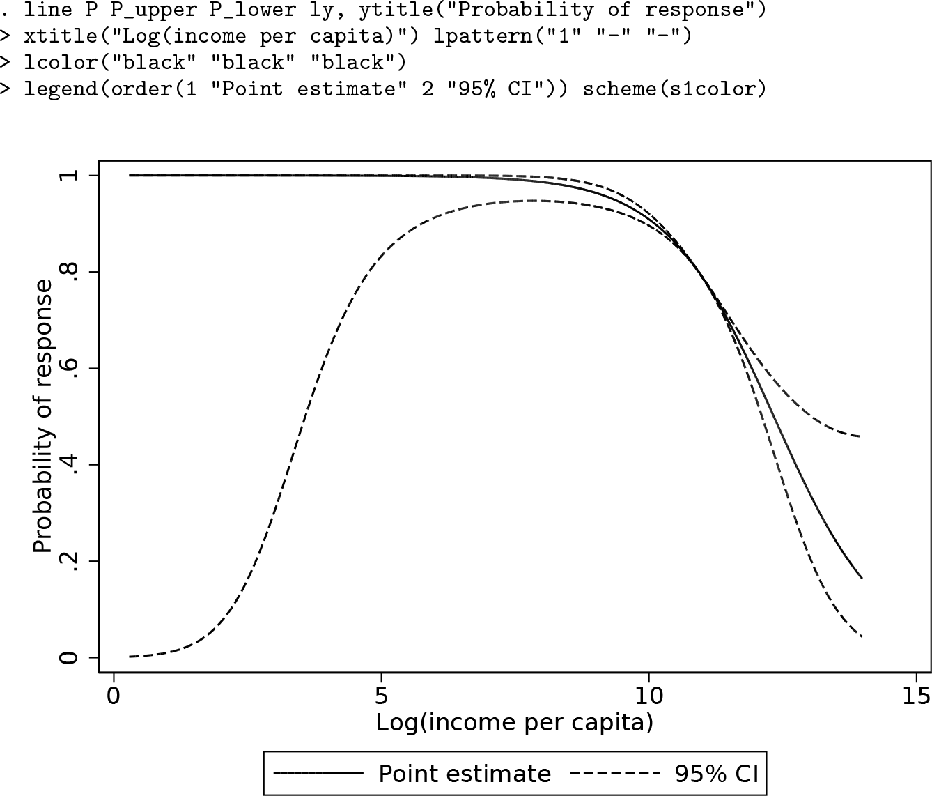
Compliance function

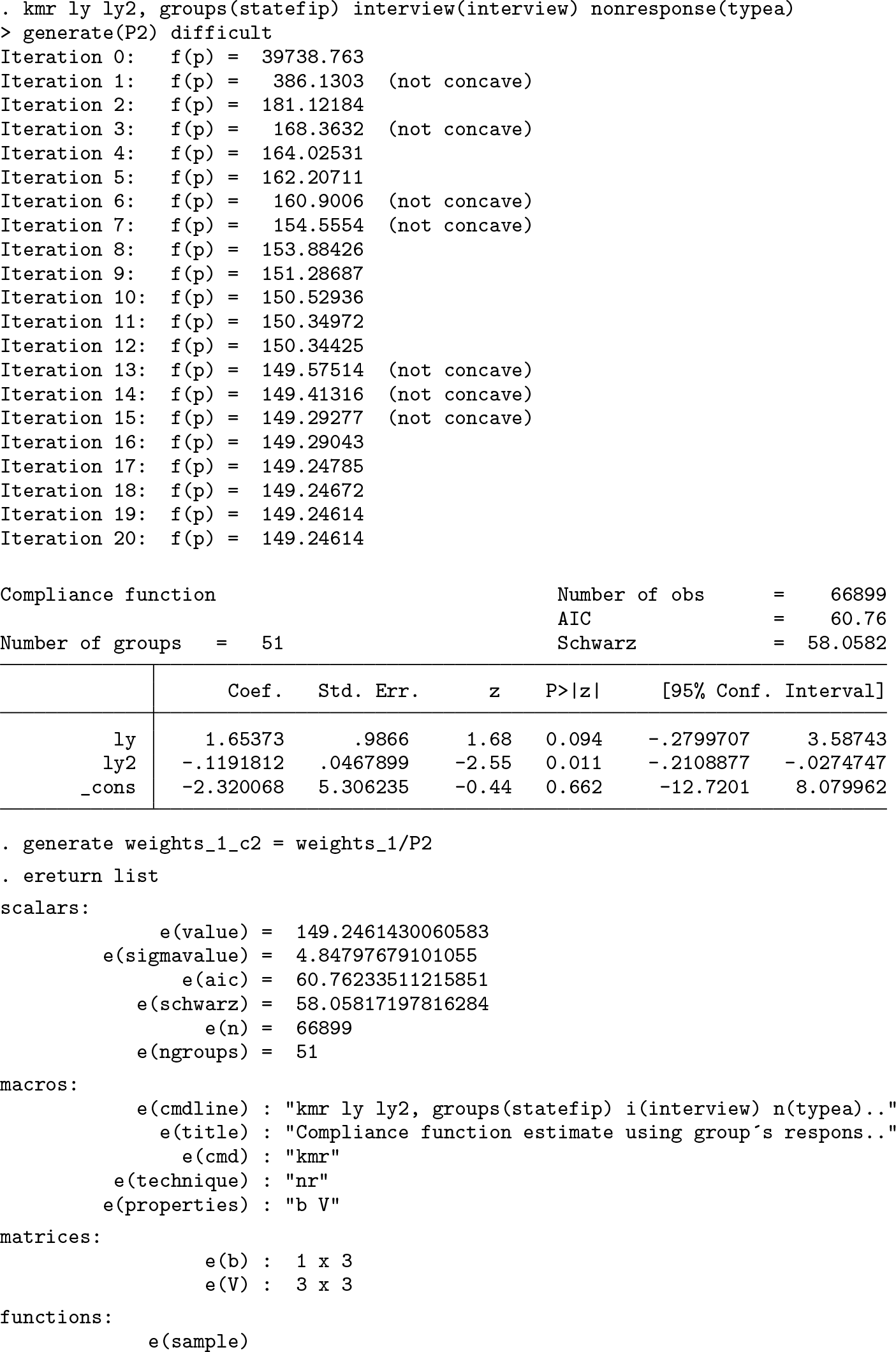
Now, we try a different specification that adds the squared log of income per capita as a second regressor. This will help to capture the fact that high nonresponse rates may occur in both tails of the income distribution, not just among rich households, as documented in Bollinger et al. (2019).

The inclusion of the log of income squared does capture some nonlinearity of compliance with respect to income. However, the estimates appear to be less precisely estimated (two of the coefficient’s p-values are below 5% confidence level). Moreover, the Akaike criterion suggests that the linear specification is preferable.

Figure 3.

Compliance function quadratic on log(income)

As we mention at the end of section 2, we can also compute the standard errors using bootstrap. We do so by defining a small program called kmrboot that resamples states with replacement and estimates the compliance function for each new sample. This program is then called 1,000 times by the command simulate, which stores the estimated coefficients in each repetition.

From the results of the bootstrap exercise, we find a level of uncertainty surrounding the parameter estimates that is similar to the standard errors previously reported, although the confidence interval is slightly wider.

Finally, we can use the community-contributed command fastgini (Sajaia 2007) to compute the Gini coefficients using the following alternatives: CPS sample weights, raw data, “grossed-up” by state, and the kmrcorrected weights according to the specification that uses log of income:

In our exercise, we derive a range of values for our corrected Gini coefficient using the point estimates of the compliance function and its upper and lower bounds derived from the 95% confidence interval (row kmr and columns Point, Lower, and Upper, respectively). We then do the same for the range of values of the compliance function derived from the bootstrap exercise (row kmrboot). We prefer this “range of values” approach to the use of standard errors obtained via the fastgini command alone because the latter would leave out a substantial source of uncertainty originating from the adjustments of the original weights.⁶

We can summarize the results as follows. The use of sample weights does not significantly change the Gini coefficient compared with the use of unweighted data (comparing the two rows, ASEC and Raw); the proposed method of weight adjustment increases the estimated Gini coefficient by at least 8.6%, going from an uncorrected Gini of 0.465 to 0.505 (comparing the two rows, ASEC and kmr). The uncertainty associated with the estimation of the compliance function is nonnegligible, and it does not change significantly when the standard errors are computed using the bootstrap method (comparing the two columns Lower and Upper).

5 Conclusion

Unit nonresponse in household surveys could lead to biases in inequality and poverty measurement. The typical methods to correct survey weights for unit nonresponse assume ignorability within some arbitrary subgroup of the population, which recent empirical evidence suggests may not hold in the case of household survey data.

In this article, we presented the kmr command, which is designed to implement the econometric method introduced by Korinek, Mistiaen, and Ravallion (2007) to estimate a survey compliance function using group level nonresponse rates, allowing us to relax the ignorability assumption.

Supplemental Material

Supplemental Material, sj-zip-1-stj-10.1177_1536867X211000025 - kmr: A command to correct survey weights for unit nonresponse using groups’ response rates

Supplemental Material, sj-zip-1-stj-10.1177_1536867X211000025 for kmr: A command to correct survey weights for unit nonresponse using groups’ response rates by Ercio Muñoz and Salvatore Morelli in The Stata Journal

Footnotes

6 Acknowledgments

We thank Carolyn Fisher for comments on the draft and Anton Korinek for providing a MATLAB code with the dataset used in their article, which greatly facilitated this project. We are also grateful for the insightful and critical comments received by two anonymous referees, which pushed us to improve the structure of the article.

7 Programs and supplemental materials

To install a snapshot of the corresponding software files as they existed at the time of publication of this article, type

Notes

References

Bollinger

C. R.

Hirsch

B. T.

Hokayem

C. M.

Ziliak

J. P.

2019. Trouble in the Tails? What We Know about Earnings Nonresponse 30 Years after Lillard, Smith, and Welch. Journal of Political Economy 127: 2143–2185. https://doi.org/10.1086/701807.

Flood

King

Rodgers

Ruggles

Warren

2018. Integrated public use microdata series, current population survey: Version 6.0 [dataset]. Minneapolis, MN: IPUMS. https://doi.org/10.18128/D030.V6.0.

Hlasny

2020. Nonresponse bias in inequality measurement: Cross-country analysis using Luxembourg Income Study surveys. Social Science Quarterly 101: 712–731. https://doi.org/10.1111/ssqu.12762.

Hlasny

Verme

2018a. Top incomes and the measurement of inequality in Egypt. World Bank Economic Review 32: 428–455. https://doi.org/10.1093/wber/lhw031.

Hlasny

Verme

2018b. Top incomes and inequality measurement: A comparative analysis of correction methods using the EU SILC data. Econometrics 6: 30. https://doi.org/10.3390/econometrics6020030.

Jann

2005. moremata: Stata module (Mata) to provide various functions. Statistical Software Components S455001, Department of Economics, Boston College. https://ideas.repec.org/c/boc/bocode/s455001.html.

Korinek

Mistiaen

J. A.

Ravallion

2006. Survey nonresponse and the distribution of income. Journal of Economic Inequality 4: 33–55. https://doi.org/10.1007/s10888-005-1089-4.

Korinek

Mistiaen

J. A.

Ravallion

2007. An econometric method of correcting for unit nonresponse bias in surveys. Journal of Econometrics 136: 213–235. https://doi.org/10.1016/j.jeconom.2006.03.001.

Meyer

B. D.

Mok

W. K. C.

Sullivan

J. X.

2015. Household surveys in crisis. Journal of Economic Perspectives 29: 199–226. https://doi.org/10.1257/jep.29.4.199.

10.

Sajaia

. 2007. fastgini: Stata module to calculate Gini coefficient with jackknife standard errors. Statistical Software Components S456814, Department of Economics, Boston College. https://ideas.repec.org/c/boc/bocode/s456814.html.

11.

Stepner

2015. maptile: Stata module to map a variable. Statistical Software Components S457986, Department of Economics, Boston College. https://ideas.repec.org/c/boc/bocode/s457986.html.

Supplementary Material

Please find the following supplemental material available below.

For Open Access articles published under a Creative Commons License, all supplemental material carries the same license as the article it is associated with.

For non-Open Access articles published, all supplemental material carries a non-exclusive license, and permission requests for re-use of supplemental material or any part of supplemental material shall be sent directly to the copyright owner as specified in the copyright notice associated with the article.

1.12 MB

0.00 MB