Implementing blopmatching in Stata

Abstract

The blopmatching estimator for average treatment effects in observational studies is a nonparametric matching estimator proposed by Díaz, Rau, and Rivera (2015, Review of Economics and Statistics 97: 803–812). This approach uses the solutions of linear programming problems to build the weighting schemes that are used to impute the missing potential outcomes. In this article, we describe blopmatch, a new command that implements these estimators.

1 Introduction

In this article, we provide an introduction to the “blopmatching” estimators for average treatment effects proposed by Díaz, Rau, and Rivera (2015) and describe blopmatch, a new command that implements these estimators.

The blopmatching approach imputes the missing potential outcome to each unit as a weighted average of observed outcomes of the units with opposite treatment, where the vector of weights is the solution of a nested pair of optimization problems. The first of these optimization problems looks for the weighting schemes that build the “synthetic covariate” defined by Abadie, Diamond, and Hainmueller (2010). Geometrically, the synthetic covariate is the projection of the covariate vector of the unit that needs imputation onto the convex hull of covariate values of the units with opposite treatment.

However, although the synthetic covariate is unique, this first optimization problem often has multiple solutions because there might be several weighting schemes building the synthetic covariate. To overcome this issue of multiplicity of solutions, the “second optimization problem” proposed by Díaz, Rau, and Rivera (2015) implements a refinement criterion for choosing one of the weighting schemes that solves the first optimization problem. More precisely, it chooses the solution that uses the covariate values of units with opposite treatment that are as close as possible to the covariate value of the unit needing imputation. Thus, blopmatching selects the weighting scheme that maximizes the unit-level covariate balance and, simultaneously, uses the units with opposite treatment with closest covariate values.

Because in the blopmatching approach the counterfactual units and the weighting scheme are determined by solving an optimization problem, it does not need an arbitrary rule to fix these parameters ex ante, a crucial aspect of most of the nonparametric approaches currently available in the literature. ¹ Finally, as Díaz, Rau, and Rivera (2015) point out, the two optimization problems involved in the blopmatching approach can be collapsed into a single linear programming program, which allows us to implement this estimator by using standard linear programming techniques.

This article is organized as follows. Section 2 presents the blopmatching estimator of average treatment effects where, in addition to presenting the general framework, a simple example illustrates what the blopmatching estimator does. Section 3 shows the procedure to estimate the marginal variances of the blopmatching estimator of average treatment effects. Section 4 details the specific method to solve the aforementioned linear program. Section 5 explains the blopmatch command, which implements the blopmatching estimators. Finally, section 6 applies blopmatch to the well-known National Supported Work Demonstration, data originally analyzed by LaLonde (1986) and later used by Dehejia and Wahba (1999).

2 Blopmatching estimator of average treatment effects

2.1 A motivating example

A simple example may be illustrative of what blopmatching does. Suppose that there are three units that are exposed to the control treatment (“control” units), whose observed outcomes are Y ₁ = Y ₁(0), Y ₂ = Y ₂(0), Y ₃ = Y ₃(0) and whose real valued covariates (continuous) are X ₁, X ₂, and X ₃, such that X ₁ < X ₂ < X ₃, so that the convex hull of these covariates is the closed interval [X ₁ , X ₃] ⊂ ℝ. Moreover, suppose that a unit that is exposed to the active treatment (“treated” unit) has observed outcome Y ₄ = Y ₄(1) ∊ ℝ and covariate X ₄ ∊ ℝ. Without loss of generality, we can assume that X ₄ ≠ X_j, j = 1, 2, 3. Here the goal is to estimate the treatment effect on this fourth unit, that is, Y ₄(1) − Y ₄(0), but the crucial complication is that Y ₄(0), the outcome of the treated unit under control treatment, is not observed. How does the blopmatching estimator impute the missing potential outcome Y ₄(0)?

Let Proj(X ₄) be the projection of X ₄ onto the closed interval [X ₁ , X ₃], that is, the nearest element of that interval to X ₄. That projection is the synthetic covariate as defined by Abadie, Diamond, and Hainmueller (2010). Notice that when X ₄ < X ₁, then Proj(X ₄) = X ₁; when X ₃ < X ₄, then Proj(X ₄) = X ₃; and when X ₄ ∊ [X ₁ , X ₃], then Proj(X ₄) = X ₄.

Regardless of the specific value of the projection, we notice now that the convex combinations of covariate values of control units generating Proj(X ₄) use vectors of weights $\lambda ={\left({\lambda }_1,{\lambda }_2,{\lambda }_3\right)}^{\text{t}}\in {ℝ}_{+}^3$ ³ that solve the following system of linear equations:

$\begin{array}{c}{\lambda }_1+{\lambda }_2+{\lambda }_3= 1\\ {\lambda }_1{X}_1+{\lambda }_2{X}_2+{\lambda }_3{X}_3= Proj(X_4)\end{array}$

1

Because in general there are multiple vectors $\lambda ={\left({\lambda }_1,{\lambda }_2,{\lambda }_3\right)}^{\text{t}}\in {ℝ}_{+}^3$ solving this linear system of equations, the solution is actually a “solution set”. Observe also that this solution set is, indeed, the solution of the next optimization problem:

$\begin{array}{c}\underset{{\left({\lambda }_1,{\lambda }_2,{\lambda }_3\right)}^{\text{t}}\in {ℝ}_{+}^3}{\min }|X_4-\sum _{j=1}^3{\lambda }_j{X}_j|\\ \text{s.t.}\\ {\lambda }_1+{\lambda }_2+{\lambda }_3= 1\end{array}$

2

Problem (2) is the first optimization problem used in the blopmatching estimator. Note that, with any weighting scheme solving this problem, we are attaining the best possible covariate balance or, alternatively, we are explaining the covariate of the treated unit through the covariates of the control units as best as possible. However, because there are more than one weighting scheme attaining the best possible covariate balance, a refinement criterion should be implemented to choose one of them. In doing this, we notice that any vector λ in that “solution set” uses covariate X_j , j = 1, 2, 3, whenever λ_j > 0. Thus, the weighted sum of distances (squared) between X ₄ and the covariates of the control units is given by

$\sum _{j=1}^3{\lambda }_j{|X_4-X_j|}^2$

The second optimization proposed by the blopmatching aims to minimize this function among the solutions of the first optimization. Hence, using (1) we see that this problem can be posed as the next linear program in terms of weights:

$\begin{array}{c}\underset{{\left({\lambda }_1,{\lambda }_2,{\lambda }_3\right)}^{\text{t}}\in {ℝ}_{+}^3}{\min }\sum _{j=1}^3{\lambda }_j{|X_4-X_j|}^2\\ \text{s.t.}\\ {\lambda }_1{X}_1+{\lambda }_2{X}_2+{\lambda }_3{X}_3= Proj(X_4)\\ {\lambda }_1+{\lambda }_2+{\lambda }_3= 1\end{array}$

3

It is clear that when X ₄ < X ₁, then the solution of (3) is λ ^b = (1, 0, 0)^t, while when X ₃ < X ₄, that solution is λ ^b = (0, 0, 1)^t. However, when Proj(X ₄) = X ₄, the solution depends on whether X ₁ < X ₄ < X ₂ or X ₂ < X ₄ < X ₃; specifically, the solution of that optimization problem is given by ${\lambda }^b={\left({\lambda }_1^b,{\lambda }_2^b,{\lambda }_3^b\right)}^{\text{t}}\in {ℝ}_{+}^3$ such that

$\{\begin{array}{l}{\lambda }_1^b=\frac{X_4-X_1}{X_2-X_1},\hspace{1em}{\lambda }_2^b=\frac{X_2-X_4}{X_2-X_1},\hspace{1em}{\lambda }_3^b=0\hspace{1em}\text{ if }\hspace{1em}{X}_1<X_4<X_2\hfill \\ {\lambda }_1^b=0,\hspace{1em}{\lambda }_2^b=\frac{X_3-X_4}{X_3-X_2},\hspace{1em}{\lambda }_3^b=\frac{X_4-X_2}{X_3-X_2}\hspace{1em}\text{ if }\hspace{1em}{X}_2<X_4<X_3\hfill \end{array}$

Thus, the blopmatching estimator imputes the missing potential outcome of the treated unit as

${\widehat{Y}}_4^b(0)={\lambda }_1^b{Y}_1+{\lambda }_2^b{Y}_2+{\lambda }_3^b{Y}_3=\{\begin{array}{llll}{Y}_1\hfill & \hspace{0.17em}\hfill & \hspace{0.17em}\hfill & \text{ if }\hspace{0.17em}\hspace{0.17em}\hspace{0.17em}{X}_4<X_1\hfill \\ Y_3\hfill & \hspace{0.17em}\hfill & \hspace{0.17em}\hfill & \text{ if }\hspace{0.17em}\hspace{0.17em}\hspace{0.17em}{X}_4>X_3\hfill \\ \left(\frac{X_4-X_1}{X_2-X_1}\right)\hfill & Y_1+\left(\frac{X_2-X_4}{X_2-X_1}\right)Y_2\hfill & \hspace{0.17em}\hfill & \text{ if }\hspace{0.17em}\hspace{0.17em}\hspace{0.17em}{X}_1<X_4<X_2\hfill \\ \left(\frac{X_3-X_4}{X_3-X_2}\right)\hfill & Y_2+\left(\frac{X_4-X_2}{X_3-X_2}\right)Y_3\hfill & \hspace{0.17em}\hfill & \text{ if }\hspace{1em}{X}_2<X_4<X_3\hfill \end{array}$

Lastly, the blopmatching estimator of the unit-level treatment effect that we wanted to estimate is given by $Y_4-{\widehat{Y}}_4^b(0)$ . In the next section, we present the extension of this simple case to a more general setting when covariates are of higher dimension.

2.2 General framework

The binary program to be evaluated is defined by the collection

${\Omega }_N= \{(X_i, Y_i, W_i)\in {ℝ}^k\times ℝ\times \{0,1\}:i\in \{1, . . . , N\left\}\right\}$

where N is the number of units, X _i ∊ ℝ ^k denotes the observed k-dimensional vector of covariates (or pretreatment variables) of unit i ∊ {1,…, N}, whose observed outcome is Y_i ∊ ℝ, and W_i ∊ {0, 1} indicates the treatment received by this unit (active treatment when W_i = 1, control treatment if W_i = 0). The number of treated units is N ₁ = ${\displaystyle \sum _{i=1}^N=W_i}$ , and the number of control units is N ₀ = N − N ₁. For the sake of simplifying the exposition of the method, the next nonrestrictive conditions are assumed throughout the article.

i) N ₀ > 1 and N ₁ > 1,

ii) W_i = 0 for i ∊ {1,…, N ₀}, and W_i = 1 for i ∊ {N ₀ + 1,…, N}.

Condition ii states that the first N ₀ units of the sample are control units, while the remaining N ₁ = N − N ₀ are the treated ones. Under condition ii, the covariate vectors of the control units are X ₁ ,…, X _{N 0}, whereas the covariate vectors of the treated units are X _{N 0 + j}, j = 1,…, N ₁.

We are interested in estimating the average treatment effect (ATE) of the program, that is, τ = $\mathbb{E}$ {Y_i (1) − Y_i (0)}, and the average treatment effect on the treated (ATT), that is, τ _tre = $\mathbb{E}$ {Y_i (1)−Y_i (0)|W_i = 1}, where Y_i (0) denotes the outcome of unit i under control treatment and Y_i (1) denotes the outcome of unit i under active treatment. In this context, Y_i (0) and Y_i (1) are called “potential outcomes” (Rubin 1974) because, for each unit, we never observe both of them in the data at hand. That is, Y_i (0) is not observed if W_i = 1 and Y_i (1) is not observed if W_i = 0. Thus, the fundamental problem of causal inference is that the missing potential outcomes must be estimated (or imputed) to estimate either the ATE or the ATT.

Throughout, the Simplex of dimension n ∊ ℕ is denoted as Δ _n = {(λ ₁ ,…, λ_n )^t ∊ ℝ₊ ⁿ : λ ₁ + · · · + λ_n = 1}. Having defined the Simplex, in this article, we are interested in the estimator of Y_i (1 − W_i ), the missing potential outcome of unit i, of the form

${\widehat{Y}}_i\left(1-W_i\right)=\{\begin{array}{ll}{\displaystyle \sum _{j=1}^{N_1}{\lambda }_{i,j}}{Y}_{N_0+j}\hfill & \text{ if }i\in \left\{1,\dots ,N_0\right\}\hfill \\ {\displaystyle \sum _{j=1}^{N_0}{\lambda }_{i,j}}{Y}_j\hfill & \text{ if }i\in \left\{N_0+1,\dots ,N\right\}\hfill \end{array}$

with λ _i = (λ _{i, 1} ,…, λ _{i,N 1})^t ∊ Δ _{N 1} when W_i = 0 and λ _i = (λ _{i, 1} ,…, λ _{i,N 0})^t ∊ Δ _{N 0} when W_i = 1.

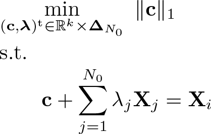
For a treated unit i ∊ {N ₀ + 1,…, N} whose Y_i (0) needs to be estimated, the blopmatching method uses the vector of weights that solves the next linear programming program, a straightforward extension of (3) to a higher dimension of the vector of covariates,

$\begin{array}{c}{\min }_{{\left({\lambda }_1,\dots ,{\lambda }_{N_0}\right)}^t\in {ℝ}_{+}^{N_0}}{\displaystyle \sum _{j=1}^{N_0}{\lambda }_j}{\Vert X_i-X_j\Vert }^2\\ \text{s.t.}\\ {\displaystyle \sum _{j=1}^{N_0}{\lambda }_j}{X}_j=\mathrm{Proj}\left(X_i\right)\\ {\displaystyle \sum _{j=1}^{N_0}{\lambda }_j}=1\end{array}$

4

where || · || denotes a given norm in the underlying vector space and Proj(X _i ) ∊ ℝ ^k is the projection of X _i onto the convex hull of covariate values of control units. It is worth recalling that the convex hull of vectors X ₁ ,…, X _{N 0} is the subset conformed by all their convex combinations. This is denoted as conv{X ₁ ,…, X _{N 0}} = {λ ₁ X ₁ + · · · +λ_{N 0} X _{N 0} : (λ ₁ ,…, λ_{N 0})^t ∊ Δ _{N 0}} ⊂ ℝ ^k . Note that Proj(X _i ) is the unique vector that complies with

$\Vert X_i-\mathrm{Proj}\left(X_i\right)\Vert ={\min }_{x\in \mathrm{conv}\left\{x_1,\dots ,x_{N_0}\right\}}\Vert X_i-X\Vert$

5

Let ${\lambda }_i^b={\left({\lambda }_{i,1}^b,\dots ,{\lambda }_{i,N_0}^b\right)}^{\text{t}}\in {\Delta }_{N_0}$ denote the solution of (4), which under continuous covariates is unique with probability one. Then, the blopmatching estimator of the missing potential outcome of treated unit i, Y_i (0), is

${\widehat{Y}}_i^b(0)={\displaystyle \sum _{j=1}^{N_0}{\lambda }_{i,j}^b}{Y}_j$

A completely analogous procedure can be presented when the unit needing imputation belongs to the control group, that is, when i ∊ {1,…, N ₀} and Y_i (1) needs to be imputed. Specifically, for that case, Δ _{N 0}, {1,…, N ₀}, and Proj(X _i ) in (4) must be replaced, respectively, by Δ _{N 1}, {N ₀ + 1,…, N}, and the projection of X _i onto the convex hull of {X _{N 0 +1} ,…, X _N }. Let ${\lambda }_i^b={\left({\lambda }_{i,1}^b,\dots ,{\lambda }_{i,N_1}^b\right)}^{\text{t}}\in {\Delta }_{N_1}$ denote the solution of the optimization problem configured for a control unit i. Then, the blopmatching estimator of its missing potential outcome, Y_i (1), is

${\widehat{Y}}_i^b(1)={\displaystyle \sum _{j=1}^{N_1}{\lambda }_{i,j}^b}{Y}_{N_0+j}$

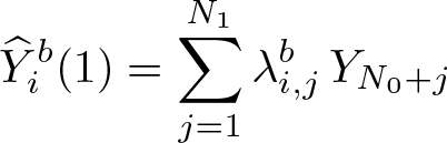
Having imputed all the missing potential outcomes, we define the blopmatching estimators of the ATE and the ATT as follows:

Definition 1. The blopmatching estimators of τ (ATE) and τ _tre (ATT) are, respectively,

$\begin{array}{l}{\widehat{\tau }}^b=\frac{1}{N}{\displaystyle \sum _{i=1}^N\left[W_i\left\{Y_i-{\widehat{Y}}_i^b(0)\right\}+\left(1-W_i\right)\left\{{\widehat{Y}}_i^b(1)-Y_i\right\}\right]}\\ {\widehat{\tau }}_{\text{tre }}^b=\frac{1}{N_1}{\displaystyle \sum _{i=1}^{N_1}\left\{Y_i-{\widehat{Y}}_i^b(0)\right\}}\end{array}$

We highlight that, to impute the missing potential outcome of any unit, the blop-matching approach does not exclude a priori any unit with opposite treatment. We also highlight that the blopmatching approach does not need to fix an exogenous number of neighbors, a crucial tuning parameter in most nonparametric approaches (see Imbens and Wooldridge [2009]).

We note now that for a treated unit i ∊ {N ₀ + 1,…, N}, the observed outcome of control unit j ∊ {1,…, N ₀} participates in the realization of ${\widehat{\lambda }}_i^b(0)$ whenever ${\widehat{\lambda }}_{i,j}^b$ is strictly positive. Because the number of equality constrains of (4) is k + 1, it follows that a “basic optimal solution” of that problem will have, at most, k+1 strictly positive components. Consequently, the number of control units whose outcomes are used when the blopmatching estimator imputes Y_i (0) should be at most k+1. We observe, however, that these units should not be necessarily the first k + 1 nearest neighbors to unit i (in terms of covariate distances); indeed, they might not even be among the first M-nearest neighbors for some fixed integer M. For instance, let k = 1, and suppose that a treated unit with covariate X_i = 1 − ⲉ, with 0 < ⲉ < 1, has to be matched against control units with covariate values X ₁ = 0, X ₂ = 1 and X_j = 1 + 1/j, j = 3,…, N ₀. In this case, ${\lambda }_i^b=(\epsilon ,1-\epsilon ,0,\dots ,0)\in {\Delta }_{N_0}$ is the solution of (4), while for ⲉ small enough, the nearest neighbors to unit i are in order of closeness: X ₂ , X_{N 0} , X_{N 0 − 1} ,…, X ₃ , X ₁. Hence, the units used to impute the missing potential outcome of X_i are its nearest and farthest neighbors.

We end this section saying that, under the assumption of strong ignorability and some additional mild conditions, Díaz, Rau, and Rivera (2015) prove that the blop-matching estimators of the ATE and ATT are consistent. We recall that the assumption of strong ignorability holds if two conditions are satisfied: unconfoundedness, which means that the treatment assignment and the potential outcomes are conditional independent given covariates (this condition is also known as selection on observed covariates); and positivity, which means that the conditional probability of being treated given covariates is strictly above zero and strictly below one (this condition is also known as overlap in the propensity score). See chapter 12 in Imbens and Rubin (2015) for a detailed discussion on observational studies under strong ignorability and chapter 21 for a procedure to assess the plausibility of this assumption in practice.

3 Estimating the marginal variance

Díaz, Rau, and Rivera (2015) propose consistent estimators of the variances of ${\widehat{\tau }}^b$ and ${\widehat{\tau }}_{\text{tre }}^b$ , whose expressions use an estimator of the conditional variance σ ²(x) = $\mathbb{V}$ (Y_i | X _i = x , W_i = w). The estimator of σ ²(x) relies on the solution of a similar optimization problem to (4). For any unit i, instead of using covariates of units belonging to the group with opposite treatment, this problem uses covariates of units in the group with the same treatment as the unit i under analysis, but of course leaving out the covariate vector of unit i. More precisely, for a treated unit i ∊ {N ₀ +1,…, N}, we denote ${\phi }_{-i}^b={\left({\phi }_1^b,\dots ,{\phi }_{i-1}^b,{\phi }_{i+1}^b,\dots ,{\phi }_{N_1}^b\right)}^{\text{t}}\in {\Delta }_{N_1-1}$ the solution of the following linear optimization problem,

$\begin{array}{c}\underset{{\left({\phi }_1,\dots ,{\phi }_{i-1},{\phi }_{i+1},\dots ,{\phi }_{N_1}\right)}^t\in {ℝ}_{+}^{N_1-1}}{\min }{\displaystyle \sum _{\begin{array}{c}j=1\\ j\ne i\end{array}}^{N_1}{\phi }_j}{\Vert X_i-X_{N_0+j}\Vert }^2\\ \text{s.t.}\\ {\displaystyle \sum _{\begin{array}{c}j=1\\ j\ne i\end{array}}^{N_1}{\phi }_j}{X}_{N_0+j}={\mathrm{Proj}}^{\star }\left(X_i\right)\\ {\displaystyle \sum _{j=1,j\ne i}^{N_1}{\phi }_j}=1\end{array}$

6

where Proj ^⋆ (X _i ) is the projection of X _i onto conv{X _{N 0 +1} ,…, X _{i − 1}, X _{i +1} ,…, X _N }. It can be shown (see Díaz, Rau, and Rivera [2015]) that the next expression is an asymptotically unbiased estimator of the conditional variance,

${\widehat{\sigma }}_i^2=\frac{{\left\{Y_i-\left({\displaystyle \sum _{j=1,j\ne i}^{N_1}{\phi }_j^b}{Y}_{N_0+j}\right)\right\}}^2}{1+{\Vert {\phi }_{-i}^b\Vert }_2^2}$

where || · ||₂ is the Euclidean norm in ℝ ^{N 1 − 1}.

For i ∊ {1,…, N ₀}, a completely analogous procedure can be implemented to obtain an estimator of the conditional variance σ ²(X _i ). Having estimated all the conditional variances, we find the following expressions to be consistent estimators (see Díaz, Rau, and Rivera [2015] for a detailed proof and the required conditions) of the marginal variances of the blopmatching estimators of the ATE and ATT,

$\begin{array}{c}\widehat{V}\left[{\widehat{\tau }}^b\right]=\frac{1}{N^2}{\displaystyle \sum _{i=1}^N\left[{\left(Y_i-{\widehat{Y}}_i^b\right)}^2+\left\{{\left(1+c_i^{[1]}\right)}^2-\left(1+c_i^{[2]}\right)\right\}{\widehat{\sigma }}_i^2\right]}-\frac{{\left({\widehat{\tau }}^b\right)}^2}{N}\\ \widehat{V}\left[{\widehat{\tau }}_{\text{tre }}^b\right]=\frac{1}{N_1^2}{\displaystyle \sum _{i=N_1+1}^N{\left(Y_i-{\widehat{Y}}_i^b\right)}^2}+\frac{1}{N_1^2}{\displaystyle \sum _{i=1}^{N_0}\left\{{\left(c_i^{[1]}\right)}^2-c_i^{[2]}\right\}}{\widehat{\sigma }}_i^2-\frac{{\left({\widehat{\tau }}_{\text{tre }}^b\right)}^2}{N_1}\end{array}$

where

$c_i^{[s]}={\displaystyle \sum _{j:W_j\ne W_i}{\left({\lambda }_{j,i}^b\right)}^s}\hspace{1em}s=1,2$

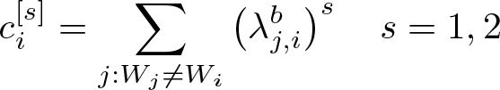
that is, the sum of weights, to the power of s, corresponding to unit i when i is used to impute the missing potential outcomes of units in the group with opposite treatment.

4 Implementation

This section presents our strategy to solve (4). Because of the similar nature of both (4) and (6), this procedure can be accommodated to solve the linear programs given by (6) and estimate the marginal variances of the treatment-effect estimators.

To solve (4), we first need to obtain the projection of X _i onto the convex hull of covariate values of units with opposite treatment condition (that is, with treatment equal to 1 − W_i ). For the sake of presentation, we initially suppose that i ∊ {N ₀ + 1,…, N} and i is a treated unit; for further convenience that will be clear later on in this section, we use Norm 1 (denoted as || · ||₁) to solve the projection problem given by (5). Here it is worth recalling that, for X = (x ₁ ,…, x_n )^t ∊ ℝ ⁿ , ||X||₁ = |x ₁ | + · · · + |x_n|. In view of these choices, we can see that (5) becomes a linear programming problem. Notice now that Proj(X _i ) is performed by the weighting schemes that solve the next optimization problem:

$\underset{\lambda ={\left({\lambda }_1,\dots ,{\lambda }_{N_0}\right)}^t\in {\Delta }_{N_0}}{\min }\Vert X_i-\left({\displaystyle \sum _{j=1}^{N_0}{\lambda }_j}{X}_j\right)\Vert$

7

Let c _i = X _i − Proj(X _i ) ∊ ℝ ^k , and let λ _i ^∗ ∊ Δ _{N 0} denote a solution to (7). Then, it is clear that (c _i, λ _i ^∗)^t ∊ ℝ ^k × Δ _{N 0} is a solution to the next optimization problem:

$\begin{array}{c}\underset{{(c,\lambda )}^t\in {ℝ}^k\times {\Delta }_{N_0}}{\min }\Vert c{\Vert }_1\\ \text{s.t.}\\ c+{\displaystyle \sum _{j=1}^{N_0}{\lambda }_j}{X}_j=X_i\end{array}$

Denoting ι _k = (1,…, 1)^t ∊ ℝ ^k and $|c|={\left(|c_1|,\dots ,|c_k|\right)}^{\text{t}}\in {ℝ}_{+}^k$ , we see that it follows directly that $\Vert c{\Vert }_1={\iota }_k^{\text{t}}|c|$ . Moreover, it is also clear that there are a couple of vectors $\alpha ,\beta \in {ℝ}_{+}^k$ such that

$c=|c|-2\beta \hspace{1em}\text{ and }\hspace{1em}c=-|c|+2\alpha$

implying that c = α − β and | c | = α + β . Consequently, $\Vert c{\Vert }_1={\iota }_k^{\text{t}}\left(\alpha +\beta \right)$ , and then

$\mathrm{Proj}\left(X_i\right)=X_i-\left({\alpha }_i^{*}-{\beta }_i^{*}\right)$

with ${\alpha }_i^{*},{\beta }_i^{*}\in {ℝ}^k$ as the corresponding components of a solution to the next linear programming problem,

$\begin{array}{c}\underset{{(\alpha ,\beta ,\lambda )}^{\text{t}}\in {ℝ}_{+}^k\times {ℝ}_{+}^k\times {ℝ}_{+}^{N_0}}{\min }{\iota }_k^{\text{t}}\alpha +{\iota }_k^{\text{t}}\beta \\ \text{s.t.}\\ \left[\begin{array}{ccccc}{I}_k& -I_k& X_1& \dots & X_{N_0}\\ 0_k^t& 0_k^{\text{t}}& 1& \dots & 1\end{array}\right]\left[\begin{array}{c}\alpha \\ \beta \\ \lambda \end{array}\right]=\left[\begin{array}{c}{X}_i\\ 1\end{array}\right]\end{array}$

8

where I _k stands for the identity matrix of ℝ ^{k × k} and 0 _k ∊ ℝ ^k is the vector with all entries zero.

In the following, $j=1,\dots ,n,e_j^n$ denotes the j-vector of the canonical basis of ℝ ⁿ . Because (8) has k + 1 equality constraints, to implement the “revised Simplex method” (see Matoušek and Gärtner [2007]) to obtain a solution, we should “mark” k + 1 linear independent (l.i) columns of the (k + 1) × (2 k + N ₀) matrix on the left-hand side of restrictions of (8) (this matrix denoted as Γ). In doing this, by setting K = {1,…, k} and denoting X _i = (X _{1 ,i},…, X_k,i )^t, we set

${\mathcal{B}}_i=\left\{s\in K:X_{s,i}\ge X_{s,N_0}\right\}\cup \left\{k+s:s\in K,X_{s,i}<X_{s,N_0}\right\}\cup \left\{2k+N_0\right\}$

It is clear that the (2k + N ₀)-column of matrix Γ, namely, the vector (X _{N 0}, 1)^t ∊ ℝ ^{k +1}, is l.i from the first 2 k columns of that matrix. It is also clear that, by construction, the columns of Γ marked by ${\mathcal{B}}_i$ \{2k+N ₀} are pairwise orthogonal. In consequence, columns of Γ marked by ${\mathcal{B}}_i$ conform a basis of ℝ ^{k +1}. To show these columns give a “basic feasible solution” for (8), we show that a solution induced by them is nonnegative. In this regard, it is easy to check that such a solution is given by $\overline{\alpha }=\left({\overline{\alpha }}_j\right)\in {ℝ}^k,\overline{\beta }=\left({\overline{\beta }}_j\right)\in {ℝ}^k$ , and $\overline{\lambda }\in {ℝ}^{N_0}$ such that

$\begin{array}{l}{\overline{\alpha }}_j=+\max \left\{X_{j,i}-X_{j,N_0},0\right\},j\in \{1,\dots ,k\}\\ {\overline{\beta }}_j=-\min \left\{X_{j,i}-X_{j,N_0},0\right\},j\in \{1,\dots ,k\}\\ \overline{\lambda }=e_{N_0}^{N_0}\end{array}$

Hence, by using the basic feasible solution above, we can solve (8) by the revised Simplex method, which gives the vector Proj(X _i ), as desired. All the commands needed for that purpose, programmed using Mata codes, are provided in addition to this article.

Having found Proj(X _i ), we can solve (4). Specifically, our commands implement the solution using either the Euclidean distance or the Mahalanobis distance (the choice is left to the researchers). In what follows, the norm is ||·||, and, without loss of generality, we present the implementation for a treated unit i ∊ {N ₀ + 1,…, N}.

We observe now that λ _i ^b = (λ^b _{i, 1} ,…, λ^b _i,N 0)^t ∊ Δ _{N 0}, which solves (4), is also a solution of the next linear optimization problem:

$\begin{array}{c}\underset{\text{λ}\in {ℝ}_{+}^{N}0}{{\displaystyle \min }}{\displaystyle {\sum }_{j=1}^{N_0}{\lambda }_j\parallel }{X}_j-X_i{\parallel }^2\\ \text{s.t.}\\ \left[\begin{array}{ccc}{X}_1& \dots & X_{N_0}\\ 1& \dots & 1\end{array}\right]\left[\begin{array}{c}{\lambda }_1\\ ⋮\\ {\lambda }_{N_0}\end{array}\right]=\left[\begin{array}{c}Proj\left(X_i\right)\\ 1\end{array}\right]\end{array}$

9

We observe also that any solution λ _i ^∗ = (λ ^∗ _{i, 1} ,…, λ ^∗ _i,N 0)^t of (7) is a feasible point for (9), although not necessarily a basic solution. Nonetheless, it is not difficult to realize that the subset

${\mathcal{C}}_i=\left\{j\in \left\{1,\dots ,N_0\right\}:{\lambda }_{i,j}^b>0\right\}$

Identifies $\#\mathcal{C}$ ≤ k + 1 linear independent columns of the coefficient matrix on the left-hand side of restrictions of (9). If we assume that N ₀ > k, N ₁ > k, and covariates are continuous, under general conditions (see Cover and Efron [1967]), then any k + 1 columns of that matrix are l.i with probability one (these columns are in “general position”). Consequently, without loss of generality, we can assume that $\mathcal{C}$ = k + 1, implying that the vector ${\lambda }_i^{\ast }$ is a basic feasible solution of (9). Using this vector, we can again implement the revised Simplex method to solve (9). ² For N ₀ ≤ k (or N ₁ ≤ k), (9) can be converted into a linear programming problem with standard form so that the revised Simplex method can be directly used with λ _i ^∗ as a basic feasible solution. To implement the blopmatch command in Stata, we programmed all the commands involved in solving this optimization problem in Mata codes.

5 The blopmatch command

5.1 Syntax

blopmatch ( ovar omvarlist ) ( tvar ) [if] [in] [weight] [ , stat options ]

ovar is a binary, count, continuous, fractional, or nonnegative outcome of interest. omvarlist specifies the covariates in the outcome model. omvarlist may contain factor variables; see [U] 11.4.3 Factor variables.

tvar must contain integer values representing the treatment levels. Only two treatment levels are allowed.

5.2 Stored results

blopmatch stores the following in e():

5.3 Example

We illustrate the use of blopmatch to estimate the average treatment effect of the National Supported Work Demonstration, a labor training program, on postintervention earnings, using data from LaLonde (1986):

Table 1 describes all variables in this dataset.

Table 1.

Description of all variables in nsw.dta

Variable	Description
treat	Treatment indicator (1 if treated, 0 otherwise)
age	Age
education	Education
black	1 if black, 0 otherwise
hispanic	1 if Hispanic, 0 otherwise
married	1 if married, 0 otherwise
nodegree	1 if no degree, 0 otherwise
re75	Earnings in 1975 (in 1978 dollars)
re78	Earnings in 1978 (in 1978 dollars)

Now we use blopmatch to estimate the average treatment effect of treat on re78. Subject distances are measured using the Mahalanobis distances defined by covariates age, education, black, hispanic, married, nodegree, and (a standardized version of) re75.

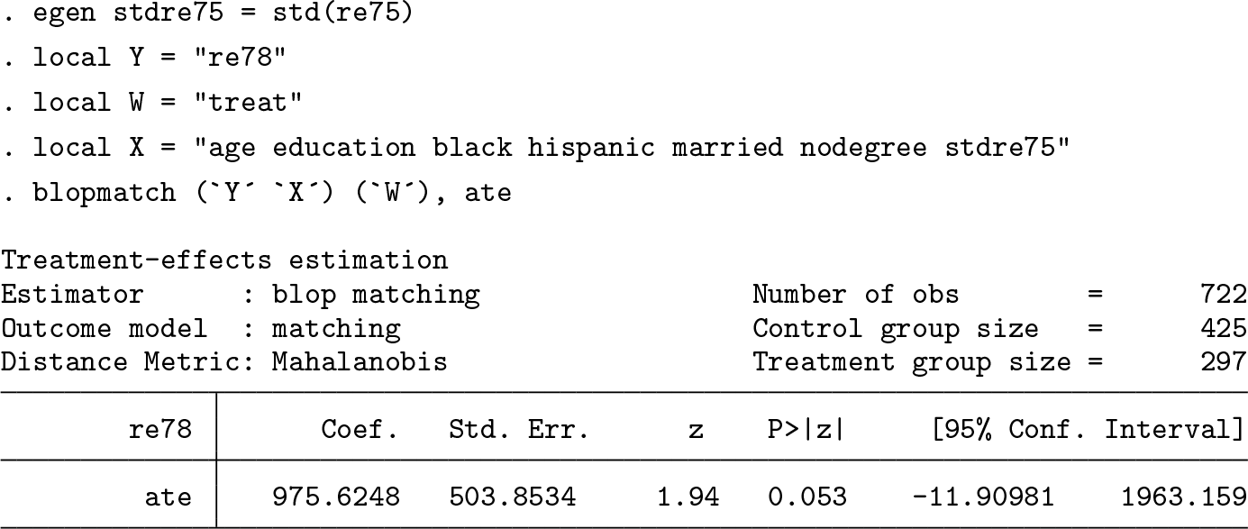
Thus, the ATE of the National Supported Work Demonstration on postintervention earnings is 975.6 USD (of 1978). In contrast, the ATE estimated with teffects nnmatch depends on the number of neighbors. For example,

Supplemental Material

Supplemental Material, sj-zip-1-stj-10.1177_1536867X211000021 - Implementing blopmatching in Stata

Supplemental Material, sj-zip-1-stj-10.1177_1536867X211000021 for Implementing blopmatching in Stata by Juan D. Díaz, Iván Gutiérrez and Jorge Rivera in The Stata Journal