Sage Journals: Discover world-class research

Abstract

Suppose that a population, composed of a minority and a majority group, is allocated into units, which can be neighborhoods, firms, classrooms, etc. Qualitatively, there is some segregation whenever allocation leads to the concentration of minority individuals in some units more than in others. Quantitative measures of segregation have struggled with the small-unit bias. When units contain few individuals, indices based on the minority shares in units are upward biased. For instance, they would point to a positive amount of segregation even when allocation is strictly random. The command segregsmall implements three recent methods correcting for such bias: the nonparametric, partial identification approach of D’Haultfœuille and Rathelot (2017, Quantitative Economics 8: 39–73); the parametric model of Rathelot (2012, Journal of Business & Economic Statistics 30: 546–553); and the linear correction of Carrington and Troske (1997, Journal of Business & Economic Statistics 15: 402–409). The package also allows for conditional analyses, namely, measures of segregation accounting for characteristics of the individuals or the units.

Keywords

st0631 segregation indices small-unit bias partial identification Duncan index Theil index Atkinson index Coworker index Gini index

1 Introduction

We consider a population made of two groups (minority and majority) whose individuals are spread across units. Units can be geographical areas, residential neighborhoods, firms, classrooms, or other clusters provided that every individual belongs to exactly one unit. We seek to measure the extent to which individuals from the minority group are concentrated in some units more than in others. Throughout the article, we follow the literature and use the word “segregation” as a neutral term to refer to such concentration. Measuring the magnitude of segregation is a necessary step to understand the underlying mechanisms and to design adequate policies.

A natural way to measure segregation is to start from the minority shares X_i/K_i , where X_i is the number of individuals from the minority group and K_i the number of individuals (or unit’s size) in unit i ∊ {1,…, n}, and then compute an inequality index based on the distribution of the proportions X_i/K_i across the n units.

There are two possible benchmarks to assess the magnitude of these indices. Evenness relates to the case where all minority shares X_i/K_i are equal across units. Randomness relates to the case where the underlying allocation assigns minority individuals at random across units. If p_i is the probability that an arbitrary individual in unit i belongs to the minority, randomness means that probabilities p_i are equal across units i. Past research has stressed the difference between both benchmarks, especially when the units are small (Cortese, Falk, and Cohen 1976). The minority share X_i/K_i is only an estimate of p_i , and even if p ₁ ,…, p_n are all equal, there will be some variation in the X_i/K_i , especially if the units’ sizes K_i are small. If one is interested in the deviations from the randomness case, indices based on minority shares, which measure the deviation from evenness, will overestimate the level of segregation. This issue is known as small-unit bias.

The problem is pervasive in applied research. For workplace and school segregation, a large share of firms have fewer than 10 employees and classrooms have usually between 20 and 40 students. The bias also arises when the units are not small per se but only surveys of individuals are available. This is the case when one attempts to measure residential segregation using the local strata of households surveys.

Two main approaches have been proposed in the literature to deal with the small-unit bias. One strand proposes to correct the so-called naive inequality indices based on the minority shares X_i/K_i . The idea was initially proposed by Cortese, Falk, and Cohen (1976) and Winship (1977) for the Duncan index. Carrington and Troske (1997, CT hereafter) extend the correction to other indices. Åslund and Skans (2009) adapt it to measure segregation conditional on covariates. Allen et al. (2015) develop another adjustment based on bootstrap. These corrections all aim at switching the benchmark from evenness to randomness by subtracting an estimate of the bias from the initial, naive index.

Another approach, adopted by Rathelot (2012, R hereafter) and D’Haultfœuille and Rathelot (2017, HR hereafter), defines segregation using an inequality index based on the unobserved probabilities p_i as a functional of the distribution F_p of p_i . In line with the rest of the literature, they assume that the X_i are independent and follow a Bin(K_i, p_i ) distribution. Conditional on K_i and p_i , R assumes a mixture of beta distributions for F_p and derives the segregation index as a function of the parameters of the distribution. HR follow a nonparametric method leaving F_p unspecified; they show that the first moments of F_p are identified under the previous binomial assumption and obtain partial identification results on the segregation measure. Both R and HR construct confidence intervals (CIs) for the segregation indices. HR also extend the methodology to study conditional segregation indices, namely, measures of “net” or “residual” segregation accounting for other covariates (either of units or individuals) that may influence allocation.

The command segregsmall allows social researchers to measure segregation in the context of small units. The command implements the methods proposed by R, HR, and CT. Conditional indices are available for all three methods. With R and HR, the command computes CIs obtained by bootstrap. Finally, the command also implements a test of the binomial assumption.

This article describes the command and presents the three methods it implements. Section 2 defines the setup and the parameters of interest and synthesizes the estimation and inference methods of R, HR, and CT. Section 3 details the syntax, options, and stored results of the segregsmall command and discusses its execution time. Section 4 presents an application of the command on French firm data to measure workplace segregation between foreigners and natives across workplaces. Section 5 concludes.

2 Setup, estimation, and inference

2.1 The setting and the parameters of interest

The population studied is assumed to be split into two groups: a group of interest, henceforth the minority group, and the rest of the population. Individuals are distributed across units. For each unit, we assume that there exists a random variable p that represents the probability for any individual belonging to this unit to be a member of the minority. The total number of individuals in a unit is denoted by K.

We now introduce the segregation indices we focus on hereafter. We consider first unconditional indices; conditional indices are introduced in section 2.6. Let us first assume that K is fixed. A segregation index θ is then a functional of the cumulative distribution function (c.d.f.) F_p of p and of m ₀₁ = E(p); that is θ = g(F_p, m ₀₁).¹ Roughly speaking, one expects such an index to be minimal when F_p is degenerate and maximal when p ∊ {0, 1}. In the former case, the probability of belonging to the minority is the same in all units, whereas in the latter case, the minority group is concentrated in a subset of units only.

The command segregsmall estimates five classical segregation indices satisfying this property; namely,

\begin{array}{l} D = \frac{\int | u - m_{01} | d F_{p} (u)}{2 m_{01} (1 - m_{01})} & (Duncan) \\ T = 1 - \frac{\int {u \ln (u) + (1 - u) \ln (1 - u)} d F_{p} (u)}{m_{01} \ln (m_{01}) + (1 - m_{01}) \ln (1 - m_{01})} & (Theil) \\ A (b) = 1 - \frac{m_{01}^{\frac{- b}{1 - b}}}{1 - m_{01}} {\int {(1 - u)}^{1 - b} u^{b} d F_{p} (u)}^{\frac{1}{1 - b}} & [Atkinson with b \in (0, 1) \\ CW = \frac{\int {(u - m_{01})}^{2} d F_{p} (u)}{m_{01} (1 - m_{01})} & (Coworker) \\ G = \frac{1 - m_{01} - \int F_{p}^{2} (u) d u}{m_{01} (1 - m_{01})} & (Gini) \end{array}

When K is random and takes values in $K, θ$ . is defin as a weighted average of indices conditional on K = k denoted $θ^{k} = g (F_{p}^{k}, m_{01}^{k})$ with $F_{p}^{k}$ the c.d.f. of p conditional on K = k and $m_{01}^{k} = E (p ∣ K = k)$ . Whether we study segregation at the unit level or at the individual level matters for the weights used. The unit-level index θ_u satisfies

θ_{u} = \sum_{k \in K} \Pr (K = k) θ^{k}

whereas the individual-level segregation index θ_i is defined by

θ_{i} = \sum_{k \in K} \frac{k \Pr (K = k)}{E (K)} θ^{k}

To estimate θ, we assume hereafter that the researcher has at his or her disposal K; however, the probability p remains unobserved. Instead, the researcher observes only X, the number of individuals belonging to the minority in the unit. By definition of p, we have E(X|K, p) = Kp, which implies that the proportion of individuals from the minority, X/K, is an unbiased estimator of p. However, because it varies conditional on p, X/K is more dispersed than p. Thus, we have for usual segregation indices including the five above,

g (F_{X / K}, m_{01}) > g (F_{p}, m_{01}) = θ

In other words, even in the absence of statistical uncertainty on the distribution of X/K, we would still overestimate the segregation index by using X/K in place of p. Moreover, this bias increases as K decreases. We refer to this issue as the small-unit bias hereafter.

The binomial assumption

We assume henceforth that individuals are allocated into units independently from each other. Namely, X is assumed to follow, conditional on p and K, a binomial distribution Bin(K, p). This assumption may be restrictive when allocation is in some way sequential and influenced by the composition of units. But more importantly, this assumption is testable (see section 2.5).

2.2 Nonparametric approach

Identification

This approach, followed by HR, leaves the distribution F_p of p unrestricted. Combined with the binomial assumption, it entails a nonparametric binomial mixture model for X. Let us first suppose that K is constant; if not, we can simply retrieve aggregated indices θ_u and θ_i using (1) and (2). We also assume that K > 1; if K = 1, the distribution of X is not informative on θ, and we get only trivial bounds on it, namely, 0 and 1 for the five indices above.

First, some algebra yields a one-to-one mapping between the distribution of X, defined by the K probabilities P ₀ = (P ₀₁ ,…, P ₀ _K ) ^′ with P ₀ _j = Pr(X = j) and the first K moments of F_p , denoted m ₀ = (m ₀₁ ,…, m ₀ _k ) ^′ ,

P_{0} = Q m_{0}

with Q the K × K matrix with generic entry (i, j) equal to $(\begin{matrix} K \\ j \end{matrix}) (\begin{array}{l} j \\ i \end{array}) {(- 1)}^{j - i}$ .

It follows that m ₀ is identified from the distribution of X; hence, any parameter depending only on m ₀ is point identified. It is the case of CW as soon as K ≥ 2. Second, there may be a single distribution F ^∗ corresponding to m ₀. This happens if (and only if) m ₀ belongs to the boundary $\partial M$ of the moment space $M$ .² Then, F ^∗ is a discrete distribution with at most L + 1 support points, where L is the integer part of (K + 1)/2. For instance, when K = 2, $M = {(m_{01}, m_{02}) \in {[0, 1]}^{2} : m_{01}^{2} \leq m_{02} \leq m_{01}}$ , because V(p) ≥ 0 and p ² ≤ p. Then, $\partial M$ corresponds to Dirac and Bernoulli distributions, for which we have, respectively, V(p) = 0 and p ² = p.

When m ₀ belongs to the interior $\overset{\circ}{M}$ of the moment space, there are infinitely many distributions F_p corresponding to m ₀. Then, unless we consider CW, θ is not identified in general. Nevertheless, HR show that the sharp-identified set on θ can be computed relatively easily under the following restriction.

Assumption 1. g(F, m₀₁) = ν (∫ h(x, m₀₁) dF (x), m₀₁) , where h and ν are continuous and ν(., m₀₁) is monotonic.

Assumption 1 fails for the Gini but is satisfied by the Duncan, the Theil, the Atkinson, and the Coworker indices. Under this condition, the bounds on ∫ h(x, m ₀₁) dF(x), and thus on θ, are attained by distributions with no more than K + 1 support points. Specifically, let $D_{m_{0}}^{K + 1}$ denote the set of distributions on [0, 1] with at most K +1 support points for which the vector of first K moments equals m ₀. Then, the sharp-identified set on θ is $[\underline{θ}, \bar{θ}]$ , with

\underline{θ} = \inf_{F \in D_{m_{0}}^{K + 1}} g (F, m_{01}) \bar{θ} = \sup_{F \in D_{m_{0}}^{K + 1}} g (F, m_{01})

The following theorem, which reproduces theorem 2.1 of HR, summarizes the previous discussion. Hereafter, we let $\underline{θ}$ and $\bar{θ}$ denote the sharp lower and upper bounds on θ, whether or not θ is point identified.

Theorem 1. – If $m_{0} \in \partial M, \underline{θ} = \bar{θ} = g (F^{*}, m_{01})$ , where F^∗ is the unique c.d.f. for which the first K moments are equal to m ₀. Moreover, F^∗ has at most L + 1 support points.

– If $m_{0} \in \overset{\circ}{M}$ and assumption 1 holds, $\underline{θ}$ and $\bar{θ}$ are defined by (3).

In the interior case, computing the bounds still requires a nonlinear optimization under constraints that are also nonlinear in the support points. Yet the problem can be further simplified under an additional assumption using the theory of Chebyshev systems. In particular, it requires that the function h in assumption 1 does not depend on m ₀₁, a condition satisfied by the Theil and Atkinson indices. Basically, for those two indices, no numerical optimization is needed to compute the bounds $\underline{θ}$ and $\bar{θ}$ . The idea behind it is that the bounds are attained by two special discrete distributions, called principal representations. The interest is that finding the principal representations boils down to obtaining the roots of specific polynomials, which is much simpler and faster than solving (3). We refer to HR for more details on that matter.

Estimation

Let us assume to have a sample (X_i ) _i ₌₁ _,…,n of independent and identically distributed variables with constant sizes equal to K > 1. Theorem 1 shows that θ is either point or partially identified, depending on whether $m_{0} \in \partial M$ or $m_{0} \in \overset{\circ}{M}$ . We follow this result to estimate ( $\underline{θ}$ , $\bar{θ}$ ). First, we estimate P ₀, and thus m ₀ = Q ⁻ ¹ P ₀, by constrained maximum likelihood. The constraints come from the binomial mixture model: $P_{0} \in P = {Q m : m \in M}$ . To compute the constrained maximum-likelihood estimator (MLE), HR show lemma 1 below. Let us define $N_{k} = \sum_{i = 1}^{n} 1 {X_{i} = k}$ , $S_{L + 1} = {(x_{1}, \dots, x_{L + 1}) : 0 \leq x_{1} < \dots < x_{L + 1} \leq 1}$ and $T_{L + 1} = {(y_{1}, \dots, y_{L + 1}) \in {[0, 1]}^{L + 1} : \sum_{k = 1}^{L + 1} y_{k} = 1}$ .

Lemma 1. The constrained MLE $\hat{P} = {({\hat{P}}_{1}, \dots, {\hat{P}}_{K})}^{'}$ satisfies

{\hat{P}}_{k} = (\begin{matrix} K \\ k \end{matrix}) \sum_{j = 1}^{L + 1} {\hat{y}}_{j} {\hat{x}}_{j}^{k} {(1 - {\hat{x}}_{j})}^{K - k} \forall k \in {1, \dots, K}

where $\hat{x} = ({\hat{x}}_{1}, \dots, {\hat{x}}_{L + 1})$ and $\hat{y} = ({\hat{y}}_{1}, \dots, {\hat{y}}_{L + 1})$ are given by

(\hat{x}, \hat{y}) = a r g m a x_{(x, y) \in S_{L + 1} \times T_{L + 1}} \sum_{k = 0}^{K} N_{k} \ln {\sum_{j = 1}^{L + 1} y_{j} x_{j}^{k} {(1 - x_{j})}^{K - k}}

Second, we estimate $(\underline{θ}, \bar{θ})$ . We first check whether $\hat{m} \in \partial M$ . A simple possibility to do so is by checking whether the unconstrained MLE $\tilde{P} = {({\tilde{P}}_{1}, \dots, {\tilde{P}}_{K})}^{'}$ satisfies $\tilde{P} = \hat{P}$ (in which case $\hat{m} \in \overset{\circ}{M}$ with probability approaching one). Note that the unconstrained MLE simply satisfies ${\tilde{P}}_{k} = N_{k} / n$ for all k.

When $\tilde{P} \neq \hat{P}$ , we simply let $\hat{\underline{θ}} = \hat{\bar{θ}} = g (\hat{F}, {\hat{m}}_{1})$ , where $\hat{F}$ is the distribution corresponding to $(\hat{x}, \hat{y})$ . We refer to this situation as the constrained case. If $\tilde{P} = \hat{P}$ , there are infinitely many distributions corresponding to $\hat{m}$ , and we estimate bounds for θ. We refer to this situation as the unconstrained case. For the Theil and Atkinson indices, the estimated bounds are obtained from the principal representations computed from $\hat{m}$ . For the Duncan index, optimization is required to obtain the estimated bounds. We obtain estimators of $\underline{θ}$ and $\bar{θ}$ by solving (3), replacing m ₀ by its estimator $\hat{m}$ . Finally, the Coworker index depends only on (m ₀₁ , m ₀₂). Thus, whether or not $\tilde{P} = \hat{P}$ , this index can be estimated directly by replacing (m ₀₁ , m ₀₂) by $({\hat{m}}_{1}, {\hat{m}}_{2})$ .

Inference

When assumption 1 holds, HR show that the estimators of the bounds are consistent: $(\hat{\underline{θ}}, \hat{\bar{θ}}) \overset{P}{\to} (\underline{θ}, \bar{θ})$ as the number of units n tends to infinity. Under additional assumptions, HR characterize their asymptotic distributions. This enables one to build valid asymptotic CIs for the index θ using a modified bootstrap procedure. The construction needs to account for the fact that the lower bound and upper bound collapse when $m_{0} \in \partial M$ (point identification), whereas they differ when $m_{0} \in \overset{\circ}{M}$ (partial identification). The underlying idea relates to the construction of CIs for partial identification (see Imbens and Manski [2004], Stoye [2009]). HR define a CI for the interior case, where only one of the two ends of the interval matters in the asymptotic coverage, and another for the boundary case. To obtain the nominal asymptotic coverage in all situations, HR define the final CI by selecting one of them according to the length of the estimated identification interval $(\hat{\bar{θ}} - \hat{\underline{θ}})$ relative to sampling error.³

Random unit size

The previous identification and estimation results can be adapted to cases where K is random and takes values in $K$ . Using the definitions of θ_u and θ_i in (1) and (2), the idea is to reason conditional on the unit size to get each θ^k , k ∊ $K$ , and replace the theoretical weights by plug-in estimators. More precisely, let $\hat{{\underline{θ}}^{k}}$ and $\hat{{\bar{θ}}^{k}}$ denote the estimators of the bounds of θ^k based on the subsample of units of size k. Let $\hat{\Pr} (K = k) = n^{- 1} \sum_{i = 1}^{n} 1 {K_{i} = k}$ and $\hat{E (K)} = n^{- 1} \sum_{i = 1}^{n} K_{i}$ . Then, the estimators of the bounds on θ_u and θ_i satisfy

\begin{array}{l} {\hat{\underline{θ}}}_{u} = \sum_{k \in K} \hat{\Pr} (K = k) {\hat{\underline{θ}}}^{k} {\hat{\bar{θ}}}_{u} = \sum_{k \in K} \hat{\Pr} (K = k) {\hat{\bar{θ}}}^{k} \\ {\hat{\underline{θ}}}_{i} = \sum_{k \in K} \frac{k \hat{\Pr} (K = k)}{\hat{E (K)}} {\hat{\underline{θ}}}^{k} {\hat{\bar{θ}}}_{i} = \sum_{k \in K} \frac{k \hat{\Pr} (K = k)}{\hat{E (K)}} {\hat{\bar{θ}}}^{k} \end{array}

Remark that as soon as for one size k the index θ^k is not point identified, the resulting aggregated index will be partially identified too. To obtain point identification of θ_u or θ_i , one must be in the constrained case for each k ∊ $K$ . This is unlikely to happen when the support of K contains very small sizes k, typically lower than 10.

As with the constant unit case, CIs for the aggregated indices θ_u and θ_i are constructed by the modified bootstrap procedure detailed in HR. The randomness of K just involves an additional step that consists in drawing K in its empirical distribution.

Assuming independence between K and p

The previous estimation and inference procedures are fully agnostic as regards possible dependence between K and p, which is a safe option when unit size may be a potential determinant of segregation. However, if one is ready to impose independence between these two variables, the identified bounds on θ_u = θ_i get closer to each other. This is because the $F_{p}^{k}$ coincide with the unconditional distribution of p. Thus, we can gather all units and identify the first K moments of F_p , with $\bar{K} = \max (K)$ . Estimation and inference are performed as in the case of constant unit size, with K replaced by $\bar{K}$ . Thus, assuming independence between $\bar{K}$ and p leads to an improvement in identification because we identify more moments. It also leads to more accurate estimators because one estimates a single vector P on the whole sample, instead of doing so on each subsample {i : K_i = k}, for all k ∊ $K$ . An important particular case occurs when only some individuals are observed in the unit (for example, survey data). Imagine units are of size (K_i ) _i ₌₁ _,…,n but that, for each unit i, only n_K,i individuals are sampled and observed. We let X_i denote the number of individuals belonging to the reference group in this subgroup of n_K,i people. As previously, X_i follows a binomial distribution Bin(n_K,i, p_i ) conditional on p_i and n_K,i . The previous results apply by simply replacing the unit size K by the number n_K of individuals observed in each unit. Moreover, in such settings, it is usually plausible to assume that the random variable n_K is independent of p conditional on the unit size because n_K depends on the survey process that, a priori, is orthogonal to the segregation phenomenon.

2.3 Parametric approach

This approach, followed by R, is like that of HR, except that it imposes a parametric restriction on F_p . Specifically, it is supposed to be a mixture of beta distributions. Combined with the binomial assumption for the conditional distribution of X, the model becomes fully parametric and thus can be estimated by maximum likelihood. The indices are therefore point identified, contrary to the nonparametric approach of HR.

A concern might be that the parametric restriction leads to invalid results when the model is misspecified. However, R shows through simulations that segregation indices associated with various distributions, both continuous and discrete, are accurately proxied by his parametric approach.

Estimation and inference

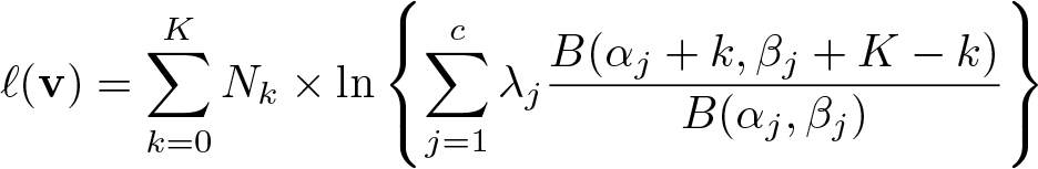
As in HR, we first assume that K is constant. Let B(., .) denote the beta function, c the number of components of the beta mixture, v = (α_j, β_j, λ_j ) _j ₌₁ _,…,c the vector of parameters with $(α_{j}, β_{j}) \in ℝ_{+}^{*} \times ℝ_{+}^{*}$ as the two shape parameters of the jth beta distribution and λ_j ∊ [0, 1] its weight $(\sum_{j = 1}^{c} λ_{j} = 1)$ . The probability density function of p distributed as a c -component mixture of beta distributions with parameters v is

f_{v} (t) = \sum_{j = 1}^{c} λ_{j} \frac{t^{α_{j} - 1} {(1 - t)}^{β_{j} - 1}}{B (α_{j}, β_{j})} \forall t \in [0, 1]

In this model, the probability that k individuals belong to the minority group can be written, after some algebra, as

\Pr_{v} (X = k) = (\begin{matrix} K \\ k \end{matrix}) \sum_{j = 1}^{c} λ_{j} \frac{B (α_{j} + k, β_{j} + K - k)}{B (α_{j}, β_{j})}

Thus, the log likelihood satisfies, up to terms independent of the parameter v,

l (v) = \sum_{k = 0}^{K} N_{k} \times \ln {\sum_{j = 1}^{c} λ_{j} \frac{B (α_{j} + k, β_{j} + K - k)}{B (α_{j}, β_{j})}}

Maximizing v ↦ ℓ(v) yields the MLE $\hat{v}$ . When we use the parametric assumption on, F_p $\hat{v}$ translates into an estimator ${\hat{F}}_{p}$ F_p of the distribution of p, which in turn yields an estimator $\hat{θ}$ of θ. The explicit expressions of the five indices above, as functions of the parameter v, are given in appendix A.1. Inference can be achieved by the delta method or by the bootstrap, performed at the unit level.

Random unit size

The adaptation to this case is exactly similar to HR method. For each k ∊ $K$ , the MLE of θ^k is obtained using the subsample of units of size k. The weights are estimated by their empirical counterparts. The estimated aggregated indices are then obtained by plug-in, using (1) and (2). When K and p are assumed independent, all units can be pooled, independently of their size, to compute the MLE of v for the whole sample. As above, the resulting estimator $\hat{v}$ allows us to estimate the distribution of p, and then θ.

2.4 Correction of the naive index

The approaches of HR and R are immune to the small-unit bias as they directly estimate g(F_p, m ₀₁). Other, previous approaches rather start from the naive index θ_N = g(F_X/K, m ₀₁) and attempt to modify it, so that the parameter becomes less sensitive to changes in K. We present here the correction proposed by CT, which is the most popular in applied work.

CT’s correction relies on the distinction between the randomness and evenness benchmarks, introduced notably by Cortese, Falk, and Cohen (1976) and Winship (1977). Evenness corresponds to X/K being constant, whereas randomness refers to the case where p is constant. Under the binomial model, however, evenness cannot occur. The central idea of CT is then to convert θ_N , which measures departure from evenness, into a distance to randomness. Let $θ_{N}^{ra}$ denote $g (F_{X^{ra}} / K, m_{01})$ , where $X^{ra} ∣ K ~ Bin {K, E (X / K)} .$ Bin{K, E(X/K)}. X ^ra /K is the proportion we would observe if p was constant and equal to E(p) = E(X/K). Then, assuming that θ ∊ [0, 1], a constraint satisfied by the five indices above, CT’s correction θ _CT is defined by $θ_{CT} = (θ_{N} - θ_{N}^{ra}) / (1 - θ_{N}^{ra})$ . CT suggest the following simulation-based estimator of θ _CT. Let $\hat{E} (p)$ denote the sample average of X/K. For s = 1,…, S, draw $X_{i, s}^{ra} ~ Bin {K_{i}, \hat{E} (p)}$ independently for each unit i. Then, letting ${\hat{F}}_{s}^{ra}$ and ${\hat{m}}_{1, s}$ denote respectively the empirical distribution and mean of ${(X_{i, s}^{ra} / K_{i})}_{i = 1, \dots, n}$ compute ${\hat{θ}}_{N, s}^{ra} = g ({\hat{F}}_{s}^{ra}, {\hat{m}}_{1, s})$ . The estimator of $θ_{N}^{ra}$ is then the mean over the S replications, ${\hat{θ}}_{N}^{ra} = $^{- 1} \sum_{s = 1}^{S} {\hat{θ}}_{N, s}^{ra}$ . Finally, ${\hat{θ}}_{CT} = ({\hat{θ}}_{N} - {\hat{θ}}_{N}^{ra}) / (1 - {\hat{θ}}_{N}^{r})$ , with ${\hat{θ}}_{N}$ the plug-in estimator of θ_N . The quantiles of ${({\hat{θ}}_{N, s}^{ra})}_{s = 1, \dots, S}$ can be used to test that the data are consistent with random allocation using randomization tests (see Boisso et al. [1994] and CT).

Links with HR and R

In general, θ _CT ≠ θ. They do coincide, however, in the extreme cases of no segregation, where p is constant, and of “full” segregation, where p follows a Bernoulli distribution. We refer to section 2.3 of R and section 2.4 of HR for further discussion on the relationship between θ _CT and θ.

2.5 Test of the binomial assumption

We have relied so far on the binomial assumption X|K, p ∼ Bin(K, p). This assumption implies that P ₀ ∊ P= {Qm : m ∊ $M$ }. A vector (m ₁ ,…, m_K ) in $M$ has to satisfy some restrictions, such as $m_{2} \geq m_{1}^{2}$ (that is, nonnegative variance). Hence, we could have Q ⁻ ¹ P ₀ ∉ $M$ if the distribution of X conditional on K and p is not binomial. In other words, the binomial assumption is testable.

HR propose a likelihood-ratio (LR) test of P ₀ ∊ P, where the constrained estimator under the null hypothesis is $\hat{P}$ , whereas the unconstrained MLE is $\tilde{P}$ . Note that these estimators are already computed to estimate $(\underline{θ}, \bar{θ})$ . For a unit size equal to k, the test statistic satisfies

{LR}_{k} = 2 \sum_{x = 0}^{k} N_{x} \ln (\frac{{\tilde{P}}_{x}}{{\hat{P}}_{x}}) = 2 \sum_{x = 0}^{k} N_{x} \ln (\frac{N_{x}}{n {\hat{P}}_{x}})

where we let $N_{x} \ln [N_{x} / (n {\hat{P}}_{x})] = 0$ if N_x = 0.

With a random unit size, the test statistic is then ${LR}_{n} = \sum_{k \in K} \hat{\Pr} (K = k) {LR}_{k}$ , where in LR _k , $N_{x} = \sum_{i = 1}^{n} I {K_{i} = k, X_{i} = x}$ . The critical values of the test are obtained by approximating the distribution of LR under the null by bootstrap. The bootstrap is performed as follows. First, we draw n units of sizes $K_{i}^{*}$ in the empirical distribution of K. Second, we draw $X_{i}^{*}$ according to ${\hat{P}}^{K_{i}^{*}}$ , where ${\hat{P}}^{k}$ is the constrained MLE of $P_{0}^{k}$ ,the distribution of X conditional on K = k. The bootstrapped test statistic LR^∗ is then computed in the sample (K_i ^∗ , X_i ^∗) _i ₌₁ _,…,n , which is drawn under the null hypothesis. For a level 1 − α ∊ (0, 1), the critical region of the test is defined by

{CR={LR>c}_{1-α} {(LR}^{*})}

with c ₁ _−α (LR^∗) the quantile of order 1 − α of LR^∗.

The results of HR imply that the test has an asymptotic level equal to α and is consistent. Remark, however, that it tests P ₀ ∊ P, which is an implication of thebinomial assumption, rather than this assumption itself. This means that the binomial assumption may fail, but P ₀ ∊ P: X|K, p could fail to be binomial, yet the distribution of X given K could be rationalized by a binomial mixture.

2.6 Conditional segregation indices

Conditional indices aim at accounting for the fact that part of the segregation along the dimension at stake may be driven by sorting according to other dimensions. In this sense, they measure the net or residual level of segregation, when the contribution of covariates to segregation is removed (see Åslund and Skans [2009]). To illustrate this point, let us consider workplace segregation between foreigners and natives. Foreigners may be hired more in some sectors of the economy on the basis of sector-specific skills. Imagine an extreme case where, within each sector, all firms hire foreigners with the same probability. As long as these probabilities differ from one sector to another, an unconditional segregation index would be positive. On the contrary, the conditional index defined in (4) below would indicate no segregation because it controls for the influence of the sector, a characteristic of units, in the allocation process. Similarly, foreigners may be hired with the same probability for all low-skilled jobs (respectively, all high-skilled jobs), but the probabilities for these two types of job may differ. In this case again, failing to account for this characteristic would lead to a positive unconditional index, while the conditional index defined in (5) below would indicate no segregation.

The previous discussion underscores that covariates can be defined either at the unit level or at the level of an individual (or of a position). We separate the two cases below because they lead to different treatments.

Unit-level covariates

Let $Z \in {1, . . ., \bar{Z}}$ denote a characteristic of a unit, which is assumed to be discrete. To account for Z in the allocation process, we measure segregation conditional on Z. For each $z \in {1, \dots, \bar{Z}}$ , let θ ₀ _z denote the segregation index we consider conditional on Z = z. The subscript 0 indicates that we consider a generic index of interest, which could correspond to either θ or θ _CT. Whatever the index, the estimation of θ ₀ _z is done exactly as in the unconditional case, focusing on the subsample {i : Z_i = z}.

The index θ ₀ _z can be of interest by itself. We can also consider an aggregate conditional index defined as follows:⁴

θ_{0, u}^{cond} = \sum_{z = 1}^{\bar{Z}} \Pr (Z = z) θ_{0 z}

The estimation of $θ_{0, u}^{cond}$ is obtained by plug-in, with $n^{- 1} \sum_{i = 1}^{n} I {Z_{i} = z}$ the empirical counterpart of Pr(Z = z). For HR and R methods, a similar bootstrap procedure as in the random size case provides asymptotic CIs for $θ_{0, u}^{cond}$ .⁵

Individual- or position-level covariates

Let $W \in {1, \dots, \bar{W}}$ denote a characteristic of an individual or of a position. To resume the example of workplace segregation, we note that a characteristic attached to individuals can be education, whereas a characteristic linked to positions can refer to the type of occupation (for example, high skilled versus low skilled). While these two forms of covariates may lead to different interpretations, they are similar as regards estimation and inference.

For each unit and each type $w \in {1, \dots, \bar{W}}$ , we suppose to observe X_w and K_w , which are respectively the number of individuals with characteristic W = w (or in positions satisfying W = w) who belong to the minority group and the overall number of individuals (or positions) of type W = w in the unit. As above, we define θ ₀ _w as the segregation index of interest conditional on W = w. With individual- or position-level covariates, the idea is to consider the subsample of individuals (or positions) such that W = w, instead of a subsample of units. Hence, θ ₀ _w can be estimated exactly as in the unconditional case simply using (X_w, K_w ) instead of (X, K).⁶

Again, θ ₀ _w might be a relevant parameter of interest on its own. Researchers can also be interested in an aggregated conditional index:

θ_{0, i}^{cond} = \sum_{w = 1}^{\bar{W}} \Pr (W = w) θ_{0 w}

The estimation of $θ_{0, i}^{cond}$ is obtained by plug-in, with $(\sum_{i = 1}^{n} K_{w i}) / (\sum_{i = 1}^{n} K_{i})$

the empirical counterpart of Pr(W = w). For HR and R methods, as previously, a modified bootstrap procedure provides asymptotic CIs for $θ_{0, i}^{cond}$ .⁷

3 The segregsmall command

The segregsmall command is compatible with Stata 14.2 and later versions.

3.1 Syntax

The syntax of segregsmall is as follows:

segregsmall varlist [if] [in] , format( format ) method( method )

[conditional( conditional ) withsingle excludingsinglepertype

independencekp repbootstrap( # ) level( # ) noci testbinomial repct( # )

atkinson( # )]

3.2 Description and main options

The command segregsmall estimates the five classical segregation indices mentioned above (Duncan, Theil, Atkinson, Coworker, and Gini) using the HR, R, or CT method. It provides CIs obtained by bootstrap in the approaches of HR and R and allows for conditional analysis for all three methods.

format( format ) indicates the format of the dataset used and needs to be either unit (datasets where an observation is a unit) or indiv (datasets where an observation is an individual). format() is required. The option determines the variables to be put in varlist. For unconditional analyses (the default without the option conditional()), these are the following:

K X for unit-level datasets; K and X correspond to the variables K and X in- troduced in section 2: the number of individuals and the number of minority individuals, respectively. K has to be strictly positive integers, and X positive or null integers. X should be lower or equal to K for each unit.

id_unit I_minority for individual-level datasets; id_unit is the identifier of the unit the individual belongs to. I_minority is a dummy variable equal to 1 when the individual belongs to the minority group, and 0 otherwise.

method( method ) specifies the method used to compute the segregation indices. method must be one of np, beta, or ct. method() is required. Argument np, standing for nonparametric, implements HR method. The command does not report the Gini index in this case, because it does not verify assumption 1. The choice beta implements R’s method assuming a beta distribution for F_p .⁸ Both methods provide estimates of the same parameters of interest, namely, θ if K is fixed and, unless independencekp is specified, (θ_u, θ_i ) if K is random. By default, they report asymptotic CIs obtained by bootstrap. With the argument ct, the command estimates the naive and CT-corrected indices θ_N and θ _CT. Confidence intervals are not computed for these parameters.

conditional( conditional ) estimates conditional segregation indices. conditional must be either unit or indiv, and it specifies the level at which the covariates included in the analysis are defined. For conditional analysis, varlist has to be

K X Z for unit-level datasets or id_unit I_minority Z for individual-level datasets, with covariates defined at unit level (unit). The variables K, X, id_unit, and I_minority are the same as in unconditional analyses. Z corresponds to the variable Z, the characteristics of units defined in section 2.6. Z needs to take values in ${1, 2, \dots, \bar{Z}}$ with $\bar{Z} \geq 2$ .

id_unit I_minority W for individual-level datasets with covariates defined at the level of individuals or any subunit level (indiv). W corresponds to the variable W, the individual (or position) characteristics introduced in section 2.6. W has to take values in ${1, 2, \dots, \bar{Z}}$ with $\bar{W} \geq 2$ .

3.3 Additional options

withsingle includes single units (with only one individual) in the analysis. As explained in section 2.2, single units are in general uninformative about the level of segregation. By default, they are not included in the data used. The option is available both for unconditional or conditional analyses.

excludingsinglepertype excludes single cells (unit × type) from the analysis. The option is relevant and available only in conditional analyses with covariates defined at the individual or subunit level. In this setting, the role of a unit in unconditional analyses is played by a cell defined as the intersection of a unit and an individual type (see section 2.6). As just described, units with only one individual are dropped by default. Yet this does not prevent the existence of single cells coming from units with more than one individual but that have only one individual of a given type W = w. Without option excludingsinglepertype, those single cells are included in the analysis, which can lead to wide estimated identified intervals in the HR method, especially when the number $\bar{W}$ of types is large. With the option, they are dropped. For consistency, the options withsingle and excludingsinglepertype are mutually exclusive.

independencekp assumes independence between K and p. The option is available only with method(np) and method(beta).

repbootstrap( # ) specifies the number of bootstrap iterations used to construct CIs in method(np) and method(beta). The default is repbootstrap(200). It is also the number of bootstrap repetitions used to test the binomial assumption.

level( # ) sets the confidence level, which has to be a scalar in (0, 1). With method(np) and method(beta), by default, the traditional 90%, 95%, and 99% confidence levels are stored (see section 3.4), and the 95% CI is displayed in Stata output. The option permits to save and display a personalized level besides (the other three are still stored). With method(ct), by default, the empirical quantiles of the index under random allocation are stored for the orders 0.01, 0.05, 0.10, 0.90, 0.95, and 0.99. The option additionally saves the empirical quantiles at order τ and 1 − τ with τ the argument of the option.

noci restricts the command to estimation: CIs are not computed. The option is applicable only to method(np) and method(beta).

testbinomial implements the test of the binomial assumption. More precisely, with method(np) and without options independencekp or noci, the test is made by default and stored: the option displays only the result in Stata output. In any other situations (method(beta) or method(ct), no CIs, or assuming K ⊥⊥ p), the option performs the test in addition to estimation and potential inference. In both cases, the number of bootstrap repetitions used for the test is the same as the one specified by option repbootstrap(). When the user wants to test the binomial assumption, we recommend always to do so combined with inference using the HR method in the general case (namely, without assuming independence between K and p): together with the test, it will give estimation and CIs from method(np) virtually for free. The option is available only in unconditional analyses.⁹

repct( # ) sets the number S of draws used to estimate θ_N ^ra in CT’s correction. Its argument needs to be a positive integer. The default is repct(50).

atkinson( # ) allows the user to specify the parameter b of the Atkinson index. Its argument has to be a real number in (0, 1). The default is atkinson(0.5); it is the only one that ensures the symmetry property for the Atkinson index (that is, the index does not change when swapping the minority and majority labels).

3.4 Stored results

The objects stored by segregsmall depend on the options, in particular, whether the analysis is unconditional or conditional. They can be gathered into three types of information about i) the data included in the analysis, ii) the method and assumptions used, and iii) the estimation and inference results.

In this section, we list the objects stored in e() by the command and detail their contents when they relate to estimation and inference results. The remaining objects have self-explanatory names and are described in the help page of the segregsmall command.

Data included in the analysis

Below, names with prefix I denote dummy variables equal to 1 if what follows is true and 0 otherwise. Objects stored in unconditional analyses are printed in black. Additional objects stored in conditional analyses are displayed in gray. The superscript *u indicates that the objects are relevant and stored only for unit-level covariates, the superscript *i for the individual-level covariates.

Method used

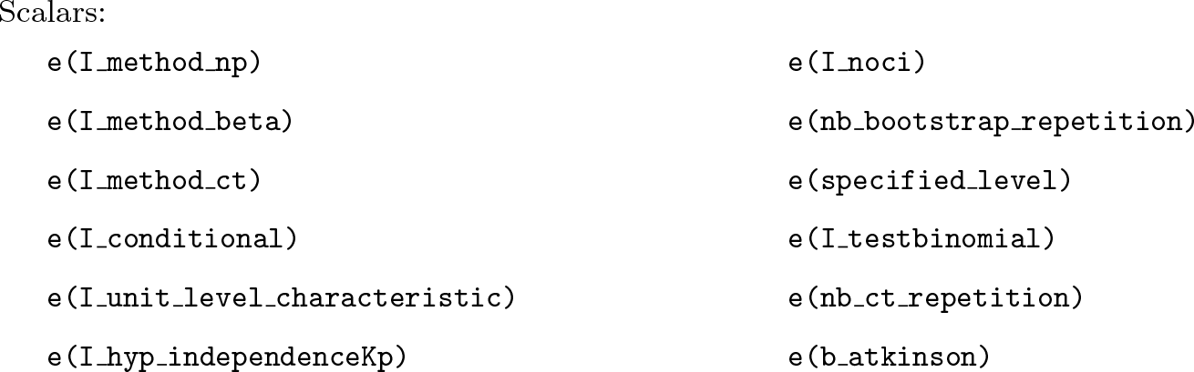
Estimation and inference

Objects relative to unconditional analyses are in black (left-hand column); those relative to conditional analyses are in gray(right-hand column). Superscripts *np and *beta indicate that objects are relevant and stored only with method(np) and method(beta).

The matrices whose name includes estimates_ci store the results of estimation and possible inference. The content of e(estimates_ci) varies with the method used but its structure remains similar. Each row corresponds to an index.

With method(beta), 10 rows represent the 2 possible aggregated indices θ_u (unitlevel weights) and θ_i (individual-level weights), when K is considered as random, for each of the 5 indices (Duncan, Theil, Atkinson, Coworker, and Gini). For each possible index weights × mapping, the columns store the estimated index using the R method with a beta distribution restriction on F_p , and asymptotic CIs at the traditional 90%, 95%, and 99% levels (plus the one specified by level() if any).

With method(np), the rows are identical, but there are only eight parameters because the Gini indices are absent. For each possible index weights × mapping, the columns of e(estimates_ci) save the estimated bounds $\hat{{\underline{θ}}_{u}}$ and ${\hat{\bar{θ}}}_{u}$ for unit-level weights (or $\hat{{\underline{θ}}_{i}}$ and ${\hat{\bar{θ}}}_{i}$ for individual-level weights); a dummy variable equal to 1 if the CI used is the boundary-case interval and 0 for the interior case; the resulting asymptotic CI at the classical 90%, 95%, and 99% levels (plus the one specified by level() if any).¹⁰

In conditional analyses, either with unit- or with individual- or position-level covariates, the matrices e(estimates_ci_aggregated) and e(estimates_ci_type_ # ) store exactly the same information as e(estimates_ci): the former for the aggregated conditional index $θ_{0, u}^{cond}$ or $θ_{0, i}^{cond}$ the latter for the index conditional on a given type #, that is θ ₀ _z with unit-level characteristics or θ ₀ _w with individual- or position-level characteristics (# ranges from z = 1 to $\bar{Z}$ or w = 1 to $\bar{W}$ ).

With method(ct), five rows correspond respectively to the Duncan, the Theil, the Atkinson, the Coworker, and the Gini indices. In columns: the naive index θ_N ; the index under random allocation ${\hat{θ}}_{N}^{ra}$ ; the CT-corrected index θ _CT; the empirical standard deviation of the draws ${({\hat{θ}}_{N, s}^{ra})}_{s = 1, \dots, S}$ under random allocation; the “standardized score” originally proposed by Cortese, Falk, and Cohen (1976), namely, $(θ_{N} - {\hat{θ}}_{N}^{ra})$ divided by that standard deviation; the empirical quantiles of ${({\hat{θ}}_{N, s}^{ra})}_{s}$ at the orders 0.01, 0.05, 0.10, 0.90, 0.95, 0.99 (τ and 1 − τ, with τ the argument of the option level() if this option is used).

e(I_constrained_case) is a dummy equal to 1 in the constrained case and 0 otherwise. As discussed in section 2.2, with random unit size, it is equal to 1 if and only if we are in the constrained case ( $D_{\hat{m}}$ restricted to a singleton) for each size k ∊ $K$ . In this case, method(np) yields point estimates for all indices. e(I_constrained_case) is identical in conditional analyses. The dummy is equal to 1 provided we are in the constrained case for each type. Otherwise, $θ_{0, u}^{cond}$ and $θ_{0, i}^{cond}$ are only partially identified with method(np).

e(test_binomial_results) is stored when the test of the binomial assumption is performed (see the option testbinomial). It is a row vector whose first element saves the value of the test statistic LR _n and the second the p-value of the test where the null hypothesis is the binomial assumption.

method(np) and method(beta) save e(info_distribution_of_p) in unconditional analyses.¹¹ This matrix contains the information learned about the distribution of p in the estimation. In the general case, without assuming K ⊥⊥ p, it means the information as regards the conditional distributions $F_{p}^{k}$ , for each k ∊ $K$ . With the option independencekp, it is about the unconditional distribution F_p .

With the method(beta) option, all the ${(F_{p}^{k})}_{k \in K}$ (or F_p when assuming K ⊥⊥ p) are supposed to follow a beta distribution. In the general case, e(info_distribution_of_p) is a matrix with $| K |$ rows. Each row is associated with a size k, and the columns report the size k; the number of units of size k in the data used, that is, $\sum_{i = 1}^{n} I {K_{i} = k}$ ; the latter quantity expressed as a proportion over the n units studied; the number of components of the beta mixture considered (that is 1); and the MLEs ${\hat{α}}_{1}$ and ${\hat{β}}_{1}$ of the two shape parameters characterizing the beta distribution assumed for F_p ^k . In the case where K ⊥⊥ p is supposed, the matrix e(info_distribution_of_p) is similar but consists of a single row because only one estimation is done, pooling all units together. It contains the maximal size $\bar{K}$ , the number of units n used for the estimation, and the estimates of the parameters that characterize the beta distribution assumed for F_p .

With the method(np) option, the structure of e(info_distribution_of_p) is more involved because the approach is nonparametric. Without the restriction K ⊥⊥ p, it contains 3 × $\bar{K}$ rows and should be read by blocks of three rows. The kth block concerns $F_{p}^{k}$ . The first line shows some general information, namely, the size k, the number of units of size k, and the proportion of such units within the data used (as in method(beta)). The most important element is displayed in the fourth column and consists of a dummy variable equal to 1 if we are in the constrained case for $F_{p}^{k}$ , that is, $\hat{m} \in \partial M$ conditional on K = k. In this case, despite the nonparametric approach, the constrained maximum-likelihood estimation yields an estimate $\hat{F}$ of $F_{p}^{k}$ which turns out to be a discrete distribution with at most ⌊(k + 1)/2⌋ + 1 support points (see section 2.2 §Estimation). In this situation, the fifth column of the first row, within the three-row block, indicates the number of support points of $\hat{F}$ , and the two following rows characterize $\hat{F}$ by reporting its support points and the corresponding probabilities. In the unconstrained case, the dummy is 0, and the two last rows, within the three-row block, are empty because there is no estimate of F_p ^k then. When assuming K ⊥⊥ p, the matrix e(info_distribution_of_p) is analogous but is made of a single three-row block because it deals only with the unconditional distribution F_p . In this case (see section 2.2 §Assuming independence between K and p), the estimation uses the first $\bar{K}$ moments of F_p . It is likely to fall in the constrained case because $\bar{K}$ will exceed 10 in most applications, a size above which simulations reveal that the probability to be in the constrained case is close to 1 even with large sample sizes n.

e(info_distribution_of_p)is interesting because virtually any segregation index is a functional of the distribution F_p [of the conditional distributions ${(F_{p}^{k})}_{k}$ in general when accounting for the randomness of K]. Consequently, an estimate of F_p [respectively of the ${(F_{p}^{k})}_{k}$ ] enables one to recover any other personalized segregation index.

3.5 Execution time

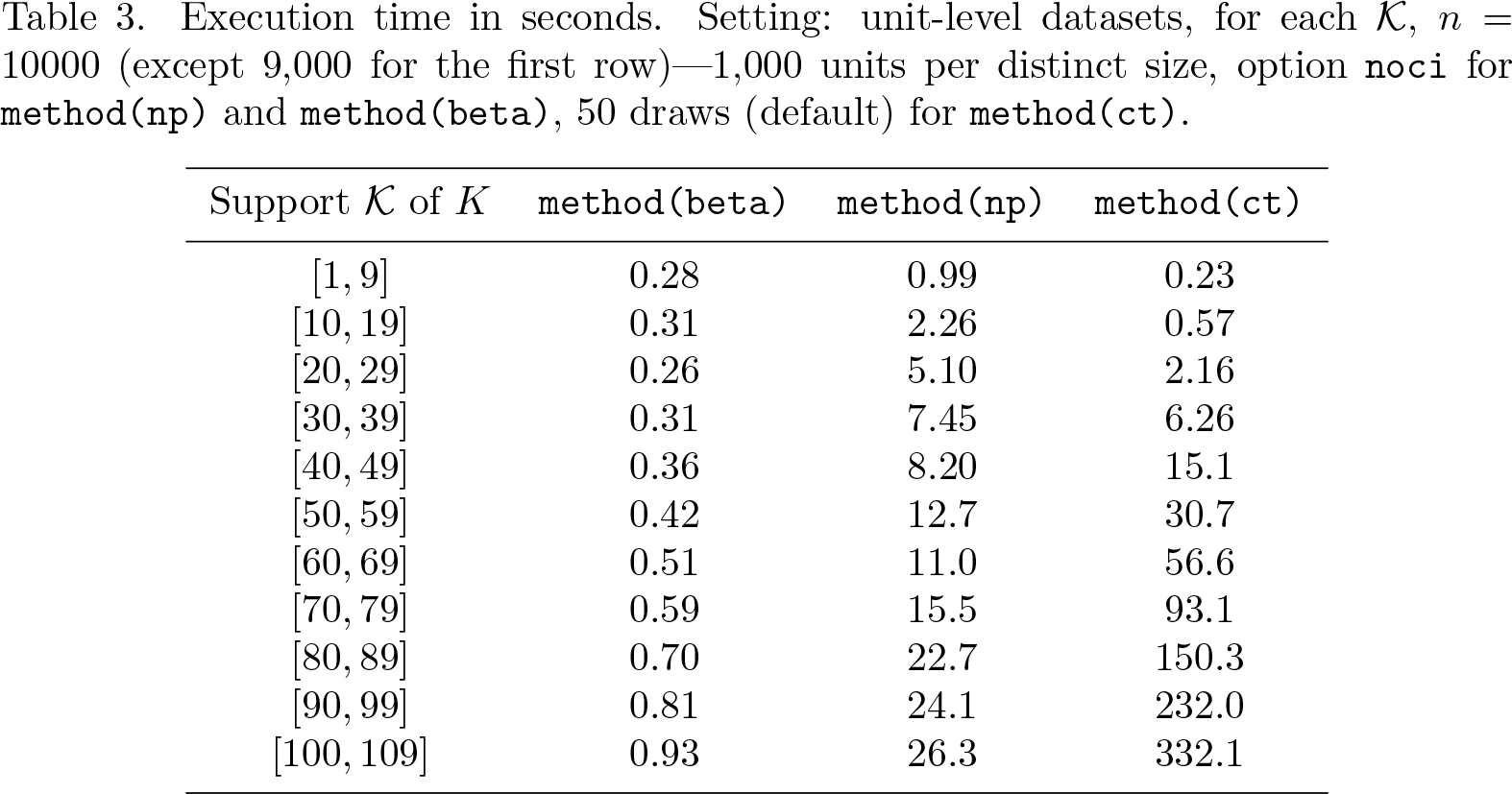
The times reported below are averaged over 50 repetitions on a desktop computer run under Windows 10 Enterprise with an Intel^® Core^TM i5-6600 CPU 3.30 GHz processor (RAM 16 Go). The operations of segregsmall can be decomposed into a preparation stage and a stage devoted to estimation and inference.

Preparation stage

The preparation stage is common to the three methods and reshapes the dataset. Its execution time is quick compared with the whole command and increases in the number n of units. For instance, with unit-level datasets, for K taking values in $K$ = [5, 15], it lasts around 0.06 second with n = 1000 and 0.99 second with n = 300000. In conditional analyses, the execution time is approximately multiplied by the number of types: for example, 6.03 seconds for 5 types and 9.17 seconds for 10 types, with $K$ = [5, 15] and n = 300000. With individual-level datasets, the preparation stage is longer because it is necessary first to form the units. With $K$ = [5, 15], it takes 0.24 seconds with 1,000 units and 9.99 seconds with 300,000 units.

Estimation and inference stage

The subsequent operations depend on the method used. The central brick of method(np) and method(beta) is the estimation of the indices for a given dataset (original or bootstrapped). The construction of CIs repeats the operation for each bootstrapped dataset. The execution time is thus more or less linear in the number of bootstrap repetitions (fixed by the option repbootstrap()). method(ct) requires one to reshuffle the data under the randomness benchmark, hence an execution time broadly linear in the number of draws (controlled by the option repct()). Table 1 illustrates this dependence for method(np) and method(beta) as well as the effect of the option conditional(). Regarding the latter, for all three methods, the same operations as in unconditional analyses are done for each type (see section 2.6). Thus, the execution time of segregsmall is roughly linear in the number of types included in the analysis.

Table 1.

Execution time in seconds. Setting: unit-level datasets, n = 300000, $K$ = [5, 15], 200 bootstrap replications, 5 types with covariates at unit level for the conditional analysis.

Analysis	Confidence intervals	method(beta)	method(np)
unconditional	no	3.2	1.3
unconditional	yes	374.2	176.9
conditional	yes	1870.8	906.8

As highlighted by table 2, the number n of units has a minor impact, mainly through the preparation stage.

Table 2.

Execution time in seconds. Setting: unit-level datasets, K = [5, 15], options independencekp and noci for method(np) and method(beta), 50 draws (default) for method(ct).

Sample size n	method(beta)	method(np)	method(ct)
1,000	0.30	2.39	0.51
10,000	0.34	2.60	0.80
50,000	0.46	2.19	0.88
100,000	0.67	2.68	1.13

The primary determinant of the computation time is the unit sizes: both the number of distinct values of the support K and the magnitude of K, as shown by table 3. With method(ct), the execution time quickly increases with the magnitude of K, while the increase is moderate for method(np) and even lighter for method(beta).¹²

Table 3.

Execution time in seconds. Setting: unit-level datasets, for each $K$ , n = 10000 (except 9,000 for the first row)—1,000 units per distinct size, option noci for method(np) and method(beta), 50 draws (default) for method(ct).

Support $K$ of K	method(beta)	method(np)	method(ct)
[1, 9]	0.28	0.99	0.23
[10, 19]	0.31	2.26	0.57
[20, 29]	0.26	5.10	2.16
[30, 39]	0.31	7.45	6.26
[40, 49]	0.36	8.20	15.1
[50, 59]	0.42	12.7	30.7
[60, 69]	0.51	11.0	56.6
[70, 79]	0.59	15.5	93.1
[80, 89]	0.70	22.7	150.3
[90, 99]	0.81	24.1	232.0
[100, 109]	0.93	26.3	332.1

4 Example

We use the command to measure workplace segregation between natives and foreigners in France (see D’Haultfœuille and Rathelot [2017] for details about the context). A large share of workers is employed in small establishments. This section shows the importance of correcting for the small-unit bias, which may lead to erroneous economic conclusions.

The data used are the 2007 Déclarations Annuelles des Données Sociales, French data linking workers to their employer. Data are exhaustive in the private sector (1.77 million establishments). In the application, we use the 1.04 million establishments that have between 2 and 25 employees. The minority group consists of individuals born outside France and with the nationality of a country outside Europe. The overall proportion of minority individuals is 4.1% in the sample studied. Figure 1 shows the estimates of workplace segregation by firm size, for the Duncan, the Theil, the Atkinson (with parameter b = 0.5), and the Coworker indices. The Gini index does not satisfy the conditions required by the nonparametric method of HR and is thus not displayed (but see figure 2 in appendix A.2 for the graph on the Gini without the nonparametric estimator).

Figure 1.

Duncan, Theil, Atkinson, and Coworker indices by firm size

The distinct methods of the package are used: the estimated bounds $\hat{\underline{θ}}$ and $\hat{\bar{θ}}$ by method(np) on θ (“np bounds”); the 95%-level CI for this parameter using the modified bootstrap procedure of method(np), with the default 200 bootstrap iterations (“np CI”); the point estimate $\hat{θ}$ by method(beta) (“beta”); the naive index θ_N (“naive”); the CT-corrected index θ _CT using method(ct), with the default 50 draws under random allocation (“ct”).

Figure 1 shows that the naive indices overestimate the actual level of segregation: they are almost always above the CI obtained by method(np) (except for the Atkinson index with K ∊ {7, 8}). This bias decreases with the size of the units. For the Duncan, the Theil, and the Atkinson indices, the estimated identification interval for θ quickly becomes informative for K ≥ 5 and reduces to a singleton for K ≥ 9 (see discussion in section 2.2). When the unit size is larger than 1, the estimated bounds of method(np) boil down to a point estimate for the Coworker index.

The point estimate $\hat{θ}$ using method(beta) is within the identification bounds of HR for the Duncan, the Theil, and the Atkinson indices, but is below HR’s CIs for the Coworker index. The CT-corrected measure θ _CT underestimates the Duncan and Theil indices, being always below the method(np)‘s CI. θ _CT lies within the CI and is quite close to the estimated identification set of θ for the Atkinson and Coworker indices.

Interestingly, the naive indices exhibit a stronger negative relationship between segregation levels and unit size than corrected ones. Neglecting the small-unit bias would produce a statistical artifact as the magnitude of the bias decreases with K and therefore would support a negative correlation while it may not be so. On the contrary, the indices that account for the small-unit bias can address this question (see section 5 of HR for further details).

Finally, we report below the Stata output obtained with the segregsmall command for method(np) and with option testbinomial. Appendix A.2 displays the output associated with method(beta)and method(ct). Compared with the analyses of figure 1 (K by K), the estimation is performed over the entire sample of units $K$ = [2, 25]) in this output without assuming K ⊥⊥ p. As detailed in section 3.3, the test of the binomial assumption is automatically performed and stored in this configuration; the option displays only the result in the Stata output. In this application, we cannot reject the binomial assumption at any standard level.

5 Conclusion

This article presented the segregsmall command which implements three methods (D’Haultfœuille and Rathelot 2017; Rathelot 2012; Carrington and Troske 1997) to measure segregation indices in settings when units (neighborhoods, firms, classrooms, etc.) contain few individuals. In such situations, naive indices overestimate the actual level of segregation and produce measures that are not comparable across settings or over time, because the small-unit bias might vary. segregsmall enables social scientists to compute segregation indices in those cases and makes the HR nonparametric approach easy to use. It provides asymptotic CIs for HR and R parameters. For all three methods, conditional indices can be estimated: they account for other covariates (either at unit level or at individual or position level) that may influence the allocation process of individuals into units and therefore measure “net” or “residual” segregation. HR and R methods can be used whatever the unit size to measure segregation as a departure from the relevant benchmark of randomness. Even with large units with above 100 individuals, the parametric approach of the R method remains quite affordable as regards computational requirements, even including inference by bootstrap.

Supplemental Material

Supplemental Material, sj-zip-1-stj-10.1177_1536867X211000018 - segregsmall: A command to estimate segregation in the presence of small units

Supplemental Material, sj-zip-1-stj-10.1177_1536867X211000018 for segregsmall: A command to estimate segregation in the presence of small units by Xavier D’Haultfœuille, Lucas Girard and Roland Rathelot in The Stata Journal

Footnotes

6 Programs and supplemental materials

To install a snapshot of the corresponding software files as they existed at the time of publication of this article, type

Notes

A Appendices

References

Allen

Burgess

Davidson

Windmeijer

2015. More reliable inference for the dissimilarity index of segregation. Econometrics Journal 18: 40–66. https://doi.org/10.1111/ectj.12039.

Aslund

Skans

O. N.

2009. How to measure segregation conditional on the distribution of covariates. Journal of Population Economics 22: 971–981. https://doi.org/10.1007/s00148-008-0189-4.

Boisso

Hayes

Hirschberg

Silber

1994. Occupational segregation in the multidimensional case: Decomposition and tests of significance. Journal of Econometrics 61: 161–171. https://doi.org/10.1016/0304-4076(94)90082-5.

Carrington

W. J.

Troske

K. R.

1997. On measuring segregation in samples with small units. Journal of Business & Economic Statistics 15: 402–409. https://doi.org/10.2307/1392486.

Cortese

C. F.

Falk

R. F.

Cohen

J. K.

1976. Further considerations on the methodological analysis of segregation indices. American Sociological Review 41: 630–637. https://doi.org/10.2307/2094840.

D’Haultfœuille

Rathelot

2017. Measuring segregation on small units: A partial identification analysis. Quantitative Economics 8: 39–73. http://doi.org/10.3982/QE501.

Imbens

G. W.

Manski

C. F.

2004. Confidence intervals for partially identified parameters. Econometrica 72: 1845–1857. https://doi.org/10.1111/j.1468-0262.2004.00555.x.

Krein

M. G.

Nudel’man

A. A.

1977. The Markov Moment Problem and Extremal Problems [in Russian]. Providence, RI: American Mathematical Society.

Rathelot

2012. Measuring segregation when units are small: A parametric approach. Journal of Business & Economic Statistics 30: 546–553. http://doi.org/10.1080/07350015.2012.707586.

10.

Stoye

2009. More on confidence intervals for partially identified parameters. Econometrica 77: 1299–1315. https://doi.org/10.3982/ECTA7347.

11.

Winship

1977. A revaluation of indexes of residential segregation. Social Forces 55: 1058–1066. http://doi.org/10.2307/2577572.

Supplementary Material

Please find the following supplemental material available below.

For Open Access articles published under a Creative Commons License, all supplemental material carries the same license as the article it is associated with.

For non-Open Access articles published, all supplemental material carries a non-exclusive license, and permission requests for re-use of supplemental material or any part of supplemental material shall be sent directly to the copyright owner as specified in the copyright notice associated with the article.

0.00 MB