
Abstract
In this article, we present the
Keywords
1 Introduction
In this article, we present the
Section 2 covers the statistical theory motivating
2 Theoretical background
2.1 Identification problem with nonrandomized treatment
Take a large population J of observationally identical individuals who face two treatment alternatives, a or b. Suppose that for each j ∊ J, potential treatment outcomes y(·) are binary: {yj
(a), yj
(b)} ∊ (0, 1) × (0, 1). A utilitarian DM faces the problem of mandating a single treatment δ ∊ (a, b) for the entire population. Before making this decision, the DM samples N individuals in J, indexed by i ∊ (1,…, N), and observes a (treatment, outcome) pair (ti, yi
) for each individual where yi
:= yi
(ti
). Let {yj
(a), yj
(b)} ∼ P , where P is the population distribution of potential outcomes. Suppose the DM draws a sample ψ ∼ Q of N pairs (ti, yi
), where Q is the sampling distribution over the sample space Ψ ⊆ ×
N
{(a, b) × (0, 1)}. We will restrict attention to the case where (ti, yi
) are independent and identically distributed so

where
With binary outcomes,

If we assume that the DM’s sampling process randomly assigns treatment t—that is,
However, if we do not make this assumption and allow nonrandomized treatment, then the DM learns nothing about Pr{y(a)|t = b} and Pr{y(b)|t = a}. The DM learns only Pr(y|t = a) and Pr(y|t = b), which equal Pr{y(a)|t = a} and Pr{y(b)|t = b}, respectively. Manski (1990) showed that when N → ∞ and Pr(t = a) ∊ (0, 1), the DM can partially identify the expected treatment effects

Even in the limiting case of no statistical imprecision, the DM’s optimal decision depends on the unobserved parameters Pr{y(a) = 1|t = b} and Pr{y(b) = 1|t = a}.
2.2 Introducing minimum MR
Formalize this decision problem under uncertainty in the manner of Wald (1949), and specify a state space S that contains all populations and sampling processes that the DM considers possible. Each state s ∊ S is characterized by a feasible pair (Ps, Qs ).
The DM can follow Bayesian decision theory and assign a prior distribution over S. However, as discussed in Manski (2004), the DM may be unable or unwilling to formulate a credible prior. Without a prior, the DM can use the maximin or minimax regret (MMR) criterion to evaluate different STRs. Following Manski (2004), we use the MMR criterion, which tries to choose an STR that yields expected welfare uniformly close to the optimal possible expected welfare across S. For further work related to MMR treatment choice, see Manski (2005, 2007a,b, 2019); Hirano and Porter (2019); Stoye (2009, 2012); Tetenov (2012); Manski and Tetenov (2016, 2019); and Kitagawa and Tetenov (2018).
To define the MMR criterion, we start by defining regret. For any STR δ and state s ∊ S, regret is the difference in ex post facto payoff between expected welfare with δ and expected welfare with the optimal choice

“max” is simply the MR that an STR δ generates over the state space:

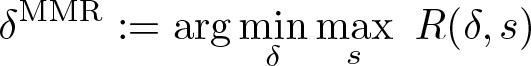
Finally, the MMR criterion chooses an STR that minimizes max regret
2.3 Asymptotically optimal STRs
When N → ∞, Manski (2020) examines the MR of two STRs: the empirical success (ES) rule and the novel asymptotic MMR (AMMR) rule. As the name suggests, the ES rule chooses δ = a if

and δ = b if the inequality is reversed. The AMMR chooses δ = a if

and δ = b if the inequality is reversed. Manski (2020) shows that the AMMR (asymptotically) minimizes MR for this decision problem and derives conditions when the ES rule does so as well. However, there are no results for the sample analogs of these or any other STRs. To fill this gap,

and δ = b if the inequality is reversed.
2.4 Computing MR
Now, we go over the algorithm for numerically computing MR for an STR δ over a feasible state space of data-generating processes. Let the s subscript of objects in step 1 denote that these are “primitives” that define state s. There are five such primitives that
The algorithm first defines a five-dimensional cube
Outline of the algorithm
0. Let the user specify a superset of the state space 1. Fix a state [Pr
s
(t = a), Pr
s
{y(a) = 1|t = a}, Pr
s
{y(b) = 1|t = b}, Pr
s
{y(b) = 1|t = a}, Pr
s
{y(a) = 1|t = b}], s ∊ 2. Given s, draw N observations 3. Repeat step 2 T times, and use the values 4. Compute approximate W (δ, Ps, Qs
) using

Compute approximate regret for δ and s:

5. Repeat steps 1–4 for each s ∊ S. 6. Return
Although the algorithm described above is simple, searching over a continuous space such as S = [0, 1]5 is intractable. Moreover, the user’s constraints C mean that the shape of S may be harder to explicitly describe than [0, 1]5. To enable feasible computation,
3 Extension to the IV setting
3.1 Classic IV (CIV) approach
A common approach to the problem of identifying

where

It follows that the DM can asymptotically point-identify
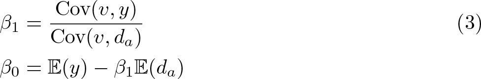
The DM would use this knowledge to assign everybody in J to treatment a if β 1 > 0 and treatment b if β 1 < 0. See Manski (2007a, chap. 7) for a textbook exposition.
3.2 Partial identification IV (PIIV) approach
In some settings, the DM may find that the assumptions of the CIV approach are not credible. The cases where the CIV approach fails are if treatment effects are heterogeneous across persons or if the instrument v is invalid [that is, Cov(v, ε) ≠ 0].
Even if the CIV approach is unsuitable, the DM can still partially identify
Suppose that v can take values in some set K. The PIIV approach begins with an assumption that

for all
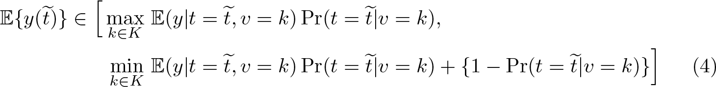
for each

If this inequality is reversed, the DM assigns treatment b to everybody in J.
3.3 IV STRs
Similarly to the ES and AMMR rules, the finite sample performance of the CIV and PIIV methods in terms of MR is unknown. To address this challenge with numerical approximation,
The framework described in sections 2.1 and 2.2 is easily extended to allow STRs that use an IV. The main difference is that there is an additional binary observable variable v, so the DM draws a sample ψ ∼ Q of N triples (ti, yi, vi
) with sample space Ψ ⊆ ×
N
{(a, b) × (0, 1) × (0, 1)}. We will restrict attention to the case where (ti, yi, vi
) are independent and identically distributed so
Now, we can construct the two built-in IV STRs using the two IV approaches described above and use MR to evaluate their performance. The CIV STR calculates the sample analog of (3),

choosing δ = a if
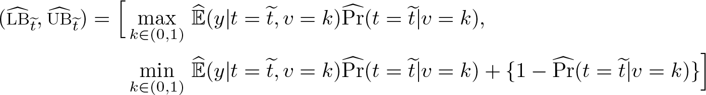
For the PIIV STR, take the sample analog of (4) to get

for each et ∊ (a, b). If
As a general result, the MR of an STR can be evaluated on any given state space. Specifically, the MR of the CIV and the PIIV STRs can be found for state spaces containing states that violate the relevant IV assumptions. One feature of
At first glance, it may be counterintuitive to examine a DM’s choice of an STR when the assumptions that motivate it are violated. Manski (2020) provides some guidance on this matter with the discussion of model choice. Although “the state space should include all states that the planner believes feasible” (Manski 2020), such a high degree of generality may preclude decision making in reality. To simplify the problem enough to allow choice, a DM might select a model as a surrogate simplified reality. A DM “using a model acts as if the model space is the state space” (Manski 2020). Therefore, a DM who uses the PIIV STR uses a model that takes the relevant IV assumption as true even if the DM suspects this assumption to be wrong in some feasible states of the world. As the statistician George Box wrote, “All models are wrong, but some are useful” (Box 1979). Therefore,
3.4 Computing MR in the IV setting
The algorithm for computing MR in the IV setting is similar to the standard algorithm described in section 2.4, except for six additional state parameters and an additional observable variable. The 6 additional state parameters mean that there are 11 state primitives (which are listed in step 1), so
Modified steps in IV algorithm
0. Let the user specify a superset of the state space 1. Fix a state [Pr
s
(t = a), Pr
s
{y(a) = 1|t = a}, Pr
s
{y(b) = 1|t = b}, Pr
s
{y(b) = 1|t = a}, Pr
s
{y(a) = 1|t = b}, Pr
s
{v = 1|t = a, y(a) = 1}, Pr
s
{v = 1|t = a, y(a) = 0}, Pr
s
{v = 1|t = b, y(b) = 1}, Pr
s
{v = 1|t = b, y(b) = 0} Pr
s
{y(a) = 1|v = 1, t = b}, Pr
s
{y(b) = 1|v = 1, t = a}], 2. Given s, draw N observations
Qualitatively, the MR algorithm for the IV setting is the same as the algorithm for the standard setting. However, the IV approach is more computationally intensive because the state space now becomes a grid over [0, 1]11 as opposed to [0, 1]5 in the standard problem. Additionally, the user can impose IV-specific constraints such as a restriction on the distribution of v, for example, Pr s {v = 1|t = k, y(a) = l} ∊ [0.01, 0.99], k ∊ (a, b), l ∊ [0, 1].
Note that although the parameters Pr s {y(a) = 1|v = 1, t = b} and Pr s {y(b) = 1|v = 1, t = a} are not used in the data simulation in step 2, they are used to check whether user-defined restrictions are satisfied in step 1. Specifically, these parameters are used to check the assumption violation restrictions described in the next section.
3.5 Restricting the violation of identifying assumptions
The default grid search includes states that violate either the CIV assumptions of y = β
0 +β
1
da
+ε and (2) or the PIIV independence assumption of
Under PIIV, an intuitive way to quantify violation is the distance

where this distance lies in [0, 1] and is 0 if the independence assumption is satisfied.
Under the CIV approach, if the model is well specified and the identifying assumptions of (2) are true, then the asymptotic IV estimator β
1 is equal to the ATE of a versus b: β
1 =

where this distance lies in [0, ∞) and is 0 if the IV estimator identifies the ATE.
4 The wald_tc command
4.1 Syntax
The syntax for
command_name specifies the name of the STR to be used. It must be either a built-in STR (see section 4.3 for details) or any user-specified STR that is written as an e-class command that returns 0 or 1 to
4.2 Options
Options to specify restrictions to the parameter space:

This could represent a setting where each sampled individual chooses t to maximize his or her own outcome. See Manski (2007a) for a discussion of this assumption, which weakens unconfoundedness.

This could represent a setting where treatment is randomized, as discussed in section 2.1. Note that specifying
Options to specify the computational details:
4.3 Built-in STRs
There are two built-in STRs for the standard framework where the STR takes data in the form (t, y) and two built-in STRs for the IV framework where the STR takes data in the form (t, y, v).
Standard STRs

Note that when the AMMR rule observes only one treatment
IV STRs

for each
If instead

4.4 Implementation details
Details on user-defined STRs
Details on option roles
The options of
Details on grid search
By default,
In addition, because the set of compound restrictions C imposes
To accommodate the Mata command
As a caveat, the use of grid search causes
Details on execution speed
In general, STRs that take in (t, y) will be much faster than IV STRs that take in (t, y, v), where the former do not have
Therefore, taking the default
To improve the speed of both IV and non-IV STRs, the user can decrease
Also, user-defined STRs will generally be much slower than built-in STRs because a user-defined STR forces
Advanced users can also improve the speed of custom STRs by adding them directly to the
Details on failure to find a solution
If the final result is an MR of 0, this means that the algorithm failed to approximate the real MR.
Additionally, this can occur if S ≠ ∅, but user-set constraints are so restrictive that each s ∊ S leaves no uncertainty for the DM, leading to a trivial problem where MR is 0.
Either of these causes may be due to the constraints alone or due to the algorithm implementation. The culprit is the constraints alone if, even abstracting from the grid search or MC simulation, the “real” state space is empty or the “real” MR is 0. In this case, the user should loosen the simple or compound parameter restrictions.
If the culprit is the algorithm interpretation, then the “real” state space may be nonempty, and the “real” MR may be larger than 0, but
A note on sample size
Users of
4.5 Stored results
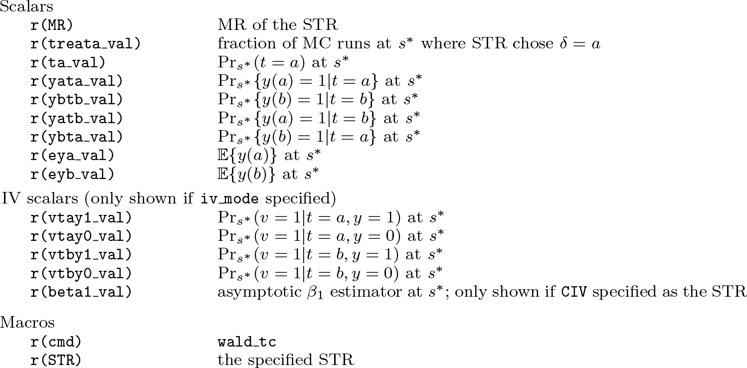
5 Examples and empirical illustration
In this section, we illustrate the functionality of
Note that after a successful execution,
5.1 Short introductory examples
Unrestricted state-space example
To run
Without strong restrictions to the state space, the ES rule will yield an MR value close to 1, which is the higher MR possible given the normalized outcomes used in
Note that the parameter space specified above contains states where Pr(t = a) ≈ 0 and Pr(t = a) ≈ 1. In this case, samples are likely to contain only t = a or t = b observations, which might be unrealistic and force the ES rule to use deterministic tiebreaking rules. To avoid this case, users can bound Pr(t = a) away from 0 and 1 using

Notice that MR has not fallen much. However, suppose we use randomized tiebreaks with option

Now, we see that MR is still high but far lower than before. In contrast, the AMMR rule performs better in an unrestricted state space, even with deterministic tiebreaks:

Unconfoundedness example
Suppose we want to impose unconfoundedness, that is, the assumption that the ATE is the same across groups. We can impose this by specifying

The imposition of unconfoundedness has slightly decreased the MR of the AMMR STR in this problem from 0.372 to 0.381.
Valid PIIV assumption example
Suppose we wish to impose the validity of the identifying assumption for the partial identification approach to IV data. We can do so by setting

Monotone treatment selection example
Suppose we would like to impose monotone treatment selection, which is relevant in a setting where individuals choose whichever treatment has a higher individual outcome. We can impose this assumption by specifying

The imposition of monotone selection leaves the MR roughly the same.
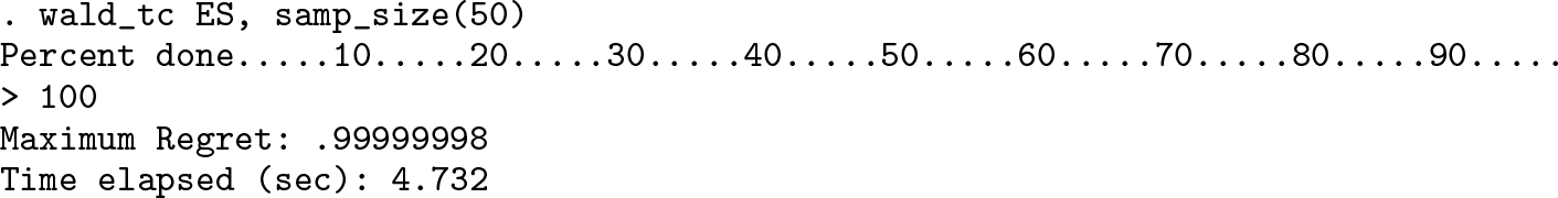
5.2 Canonical status quo versus innovation example
Here we examine a setting where the DM must choose between a status quo treatment a or an innovation b for the population after recording a sample of N = 50 treatments and outcomes in an observational study. We will examine a setting where we (as the user) know that the expected treatment effect of a is 0.5. This maps to

We get an MR of 0.398. Suppose we are interested in the state that generates this regret. We run

Although
Now, let us evaluate the AMMR STR:

We see that AMMR performs better by yielding a smaller MR of approximately 0.298. Examining

We get a similar MR of 0.292 and
Suppose that the result of

Now, we get a lower MR than before. As for AMMR:

We also get a lower MR than before, but the gap between the MR of ES and AMMR has narrowed to 0.014 from 0.1. This is due to the
Demonstrating a user-defined function
Suppose we want to evaluate the performance of a DM who uses a canonical one-sided t test with α = 0.05 to choose a treatment. Because this STR is not a built-in function, the user would have to specify a user-defined function to
The t test STR takes the following null and alternate hypotheses:

If the STR rejects the null at a α = 0.05 level, it will choose δ = b; otherwise, it will choose δ = a. Running this STR with the same parameters as before, we obtain

We see that the MR of this STR is only marginally better than that of the ES STR. Examining
In terms of implementation, this run is around 500 times slower than our previous runs. This is due to the issue of having to run the STR in Stata for each MC sample as opposed to keeping all the computation in Mata. For example, when we modify the

This run is clearly much faster and is comparable with the speed of other built-in STRs. Moreover,
5.3 Swan–Ganz catheterization example
In this section, we will demonstrate the functionality of Our primary substantive finding is that catheterization improves mortality outcomes only in the short run, if at all, and in most cases we cannot rule out that it increases mortality in the long run.
To reach their findings, Bhattacharya, Shaikh, and Vytlacil (2012) use data that record whether a patient receives a catheter (t = b) or not (t = a), whether a patient dies within a specified time after admission (y = 0) or not (y = 1), and an IV indicating whether the patient is admitted on a weekend or a weekday. The authors claim that this is a valid instrument because mortality is uncorrelated with the day of admission, while patients admitted on a weekday are about four to eight percentage points more likely to be catheterized (Bhattacharya, Shaikh, and Vytlacil 2012).
Suppose that in this setting, a DM uses some another instrument v to try to find a more definitive result regarding the treatment effect of catheterization for a population. Suppose that the DM observes a sample (N = 100) and must choose between requiring that all relevant patients receive catheters (δ = a) or none do (δ = b). We will now demonstrate how
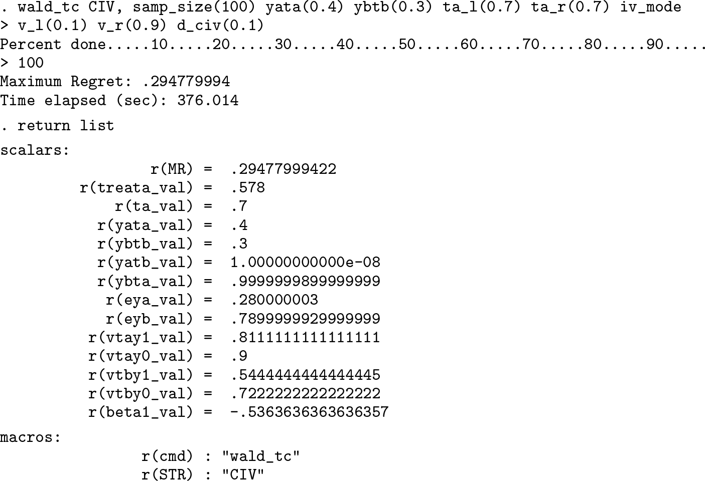
CIV STR
Suppose we know that in our population, catheterization is somewhat common but associated with worse observable outcomes, with the following parameters:

Suppose that we also believe our instrument v has a nonzero population variance [conditional on (t, y)]. To specify this concretely, we can tighten

Then, analyzing the state, we get

Therefore, at s ∗, we have that v is weakly correlated with t but has higher correlation with y, giving a β 1 that is much higher than the true treatment effect! Such a state is more likely to yield samples that would call the validity and strength of v into question. Thus, we might want to impose an upper bound on D CIV, such as 0.1. Adding this bound, we get
Compared with the original run, MR is negligibly lower,
However, there are other interesting assumptions that can change the performance of STRs, such as a monotone selection assumption. In addition to reporting that catheterized patients tend to be more severely ill than noncatheterized patients, Bhattacharya, Shaikh, and Vytlacil (2012) suggest that their findings may be due to a selection story: catheterization can be lifesaving for the most severely ill patients in the short term (that is, seven days) but cannot overcome their latent health problems in the long term.
PIIV STR
Now, let us see what happens when we run the original parameterization with the PIIV STR:
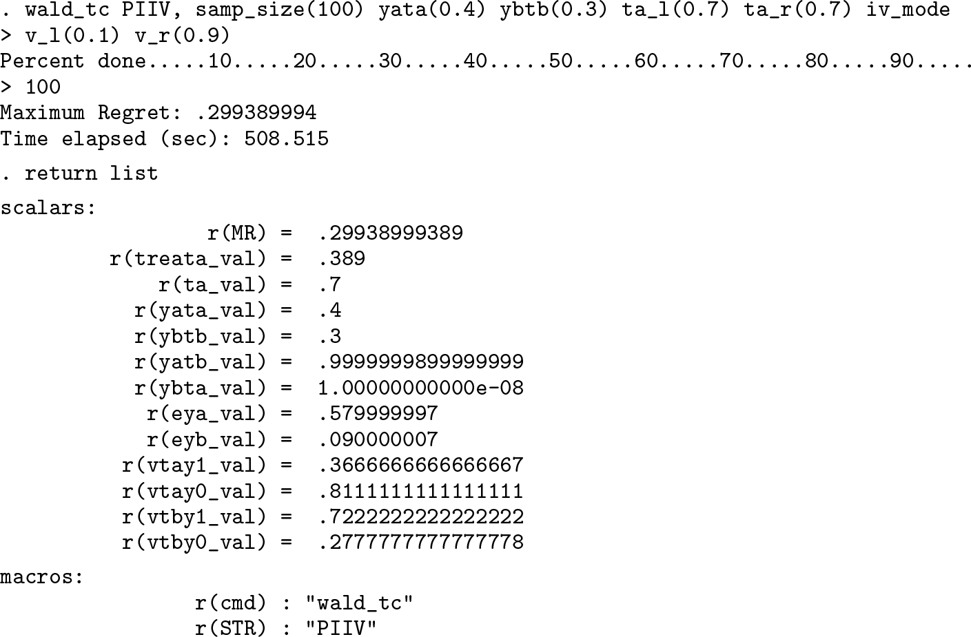
We have a similar regret to the CIV STR, although the state s ∗ is somewhat different and PIIV has a lower probability of choosing δ = a in its s ∗.
All of these examples shown above demonstrate a small fraction of the flexible options that the user has in exploring the performance of STRs under different settings of nonrandomized treatment.
Supplemental Material
Supplemental Material, sj-zip-1-stj-10.1177_1536867X211000006 - Evaluating the maximum regret of statistical treatment rules with sample data on treatment response
Supplemental Material, sj-zip-1-stj-10.1177_1536867X211000006 for Evaluating the maximum regret of statistical treatment rules with sample data on treatment response by Valentyn Litvin and Charles F. Manski in The Stata Journal
Footnotes
6 Acknowledgments
We are grateful to Aleksey Tetenov and Eduardo Campillo-Betancourt for their comments.
7 Programs and supplemental materials
To install a snapshot of the corresponding software files as they existed at the time of publication of this article, type
References
Supplementary Material
Please find the following supplemental material available below.
For Open Access articles published under a Creative Commons License, all supplemental material carries the same license as the article it is associated with.
For non-Open Access articles published, all supplemental material carries a non-exclusive license, and permission requests for re-use of supplemental material or any part of supplemental material shall be sent directly to the copyright owner as specified in the copyright notice associated with the article.