Sage Journals: Discover world-class research

Abstract

We introduce three new commands—nop, ziop2, and ziop3—for the estimation of a three-part nested ordered probit model, the two-part zero-inflated ordered probit models of Harris and Zhao (2007, Journal of Econometrics 141: 1073–1099) and Brooks, Harris, and Spencer (2012, Economics Letters 117: 683–686), and a three-part zero-inflated ordered probit model of Sirchenko (2020, Studies in Nonlinear Dynamics and Econometrics 24: 1) for ordinal outcomes, with both exogenous and endogenous switching. The three-part models allow the probabilities of positive, neutral (zero), and negative outcomes to be generated by distinct processes. The zero-inflated models address a preponderance of zeros and allow them to emerge in different latent regimes. We provide postestimation commands to compute probabilistic predictions and various measures of their accuracy, to assess the goodness of fit, and to perform model comparison using the Vuong test (Vuong, 1989, Econometrica 57: 307–333) with the corrections based on the Akaike and Schwarz information criteria. We investigate the finite-sample performance of the maximum likelihood estimators by Monte Carlo simulations, discuss the relations among the models, and illustrate the new commands with an empirical application to the U.S. federal funds rate target.

Keywords

st0625 nop ziop2 ziop3 ordinal outcomes zero inflation nested ordered probit zero-inflated ordered probit endogenous switching Vuong test federal funds rate target

1 Introduction

We introduce the commands nop, ziop2, and ziop3, which fit the two-level nested and zero-inflated ordered probit (OP) models for ordinal outcomes, including the zero- and middle-inflated OP models of Harris and Zhao (2007), Bagozzi and Mukherjee (2012), Brooks, Harris, and Spencer (2012), and Sirchenko (2020). The rationale behind the two-level nested decision process is standard in discrete-choice modeling when the set of alternatives faced by a decision-maker can be partitioned into subsets (or nests) with similar alternatives correlated because of common unobserved factors. The choice among the nests and the choice among the alternatives within each nest can be driven by different sets of observed and unobserved factors (and common factors can have different weights).

In unordered categorical data, in which choices can be grouped into the nests of similar options, the nested logit model is a popular method. Nested models for ordinal data are rare though the rationale behind them is similar: choosing among a negative response (decrease), a neutral response (no change), or a positive response (increase) is quite different from choosing the magnitude of a negative or positive response; and choosing the magnitude of a negative response can be driven by quite different determinants than choosing the magnitude of a positive response. This leads to three implicit decisions: an upper-level regime decision (a choice among the nests) and two lower-level outcome decisions (the choices of the magnitude of the negative and positive responses). See the top left panel of figure 1.

Figure 1.

Decision trees of nested and zero-inflated ordered probit models.

Furthermore, it would be reasonable for the zero (no-change) alternative to be in three nests: its own, one with the negative responses, and one with the positive responses. Hence, some zeros can be driven by similar factors as the negative or positive responses. This leads to a three-part cross-nested model with the nests overlapping at the zero response; hence, the probability of zeros is “inflated”. Because the regime decision is not observable, the zeros are observationally equivalent—it is never known to which of the three nests the observed zero belongs. Several types of models with overlapping nests for unordered categorical responses have been developed (Vovsha 1997; Wen and Koppelman 2001). Cross-nested models for ordinal outcomes are rare (Small 1987).

The prevalence of status quo, neutral, or zero outcomes is observed in many fields, including economics, sociology, technometrics, psychology, and biology. The heterogeneity of zeros is widely recognized—see Winkelmann (2008) and Greene and Hensher (2010) for a review. Studies identify different types of zeros, such as no visits to a doctor due to good health, iatrophobia, or medical costs; no illness due to strong immunity or lack of infection; no children due to infertility or choice. In the studies of survey responses using an odd-point Likert-type scale, where the respondents must indicate a negative, neutral, or positive attitude or opinion, the heterogeneity of indifferent responses (a true neutral option versus an undecided, or ambivalent, or uninformed one, commonly reported as neutral) is also well recognized and sometimes labeled as the middle category endorsement or inflation (Bagozzi and Mukherjee 2012; Hernández, Drasgow, and Gonzáles-Romá 2004; Kulas and Stachowski 2009).

Two-part zero-inflated models, developed to address the unobserved heterogeneity of zeros, combine a binary choice model for the probability of crossing the hurdle (to participate or not to participate; to consume or not to consume) with a count or ordered-choice model for nonnegative outcomes above the hurdle: the two parts are estimated jointly, and zero observations can emerge in both parts. The two-part zero-inflated models include the zero-inflated Poisson (Lambert 1992), negative binomial (Greene 1994), binomial (Hall 2000), and generalized Poisson (Famoye and Singh 2003) models for count outcomes, and the zero-inflated OP model (Harris and Zhao 2007) and zero-inflated proportional odds model (Kelley and Anderson 2008) for nonnegative ordinal responses.¹

The model of Harris and Zhao (2007) is suitable for explaining decisions such as the levels of consumption, when the upper hurdle is naturally binary (to consume or not to consume), the responses are nonnegative, and the inflated zeros are situated at one end of the ordered scale (see the bottom left panel of figure 1). Bagozzi and Mukherjee (2012) and Brooks, Harris, and Spencer (2012) modified the model of Harris and Zhao (2007) and developed the middle-inflated OP model for an ordinal outcome, which ranges from negative to positive responses, and where an abundant outcome is situated in the middle of the choice spectrum (see the bottom right panel of figure 1).

The three-part zero-inflated OP model (see the top right panel of figure 1) introduced in Sirchenko (2020) is a natural generalization of the models of Harris and Zhao (2007), Bagozzi and Mukherjee (2012), and Brooks, Harris, and Spencer (2012). A trichotomous regime decision is more realistic and flexible than a binary decision (change or no change) if applied to ordinal data with negative, zero, and positive values.

2 Models

2.1 Notation and assumptions

The observed dependent variable y_t , t = 1, 2,…, T, is assumed to take on a finite number of ordinal values j coded as {−J ⁻ ,…, −1, 0, 1,…, J ⁺}, where a potentially heterogeneous (and typically predominant) response is coded as 0. The latent unobserved (or only partially observed) variables are denoted by “∗”. Each model assumes an ordered-choice regime decision and the ordered-choice outcome decisions conditional on the regime. The regime decision can be correlated with each outcome decision. We denote the following: by x _t , $x_{t}^{-}, x_{t}^{+},$ and z _t , the tth rows of the observed data matrices (which in addition to the predetermined explanatory variables may also include the lags of y_t ); by β , β ⁻, β ⁺, and γ , the vectors of slope parameters; by α , α ⁻, α ⁺, and µ , the vectors of threshold parameters; by ρ , ρ ⁻, and ρ ⁺, the correlation coefficients; by ε_t , $ε_{t}^{-}, ε_{t}^{+},$ and ν_t , the error terms that are independent and identically distributed (i.i.d.) across t with normal cumulative distribution function (CDF) Φ with 0 means and variances σ ², $σ_{-}^{2}, σ_{+}^{2},$ and $σ_{ν}^{2},$ respectively; and by $Φ_{2} (g_{1}; g_{2}; σ_{1}^{2}; σ_{2}^{2}; ρ),$ the CDF of the bivariate normal distribution of the two random variables g ₁ and g ₂ with 0 means, variances $σ_{1}^{2}$ and $σ_{2}^{2},$ and correlation coefficient ρ.

\begin{matrix} Φ_{2} (g_{1}; g_{2}; σ_{1}^{2}; σ_{2}^{2}; ρ) = \frac{1}{2 π σ_{1} σ_{2} \sqrt{1 - ρ^{2}}} \\ \int_{- \infty}^{g_{1}} \int_{- \infty}^{g_{2}} \exp {- \frac{u^{2} / σ_{1}^{2} - 2 ρ u w / σ_{1} σ_{2} + w^{2} / σ_{2}^{2}}{2 (1 - ρ^{2})}} d u d w \end{matrix}

2.2 Three-part nested ordered probit model

Despite the widespread use of nested logit models for unordered categorical responses, we are aware of only one example of the nested OP model in the literature (Sirchenko 2020). The two-level nested ordered probit (NOP) model can be described as

\begin{array}{l} Upper-level decision: & r_{t}^{*} = z_{t} γ + ν_{t}, s_{t} = {\begin{array}{r} 1 & if & μ_{2} < r_{t}^{*} \\ 0 & if & μ_{1} < r_{t}^{*} \leq μ_{2} \\ - 1 & if & r_{t}^{*} \leq μ_{1} \end{array} \\ Lower-level decisions & \begin{array}{l} y_{t}^{- *} = x_{t}^{-} β^{-} + ε_{t}^{-}, y_{t}^{+ *} = x_{t}^{+} β^{+} + ε_{t}^{+} \\ y_{t} = {\begin{array}{l} j (j > 0) & if & s_{t} = 1 and α_{j - 1}^{+} < y_{t}^{+ *} \leq α_{j}^{+} \\ 0 & if & s_{t} = 0 \\ j (j < 0) & if & s_{t} = - 1 and α_{j}^{-} < y_{t}^{- *} \leq α_{j + 1}^{-} \end{array} \\ \begin{array}{l} where - \infty = α_{0}^{+} \leq α_{1}^{+} \leq \dots \leq α_{J^{+}}^{+} = \infty \\ and - \infty = α_{- J^{-}}^{-} \leq α_{- J^{-} + 1} \leq \dots \leq α_{0}^{-} = \infty \end{array} \end{array} \\ Correlation among decisions: & [\begin{matrix} ν_{t} \\ ε_{t}^{i} \end{matrix}] \overset{i.i.d.}{\sim} N (\begin{matrix} 0 \\ 0 \end{matrix}, [\begin{matrix} σ_{ν}^{2} & ρ^{i} σ_{ν} σ_{i} \\ ρ^{i} σ_{ν} σ_{i} & σ_{i}^{2} \end{matrix}]), i \in {-, +} \end{array}

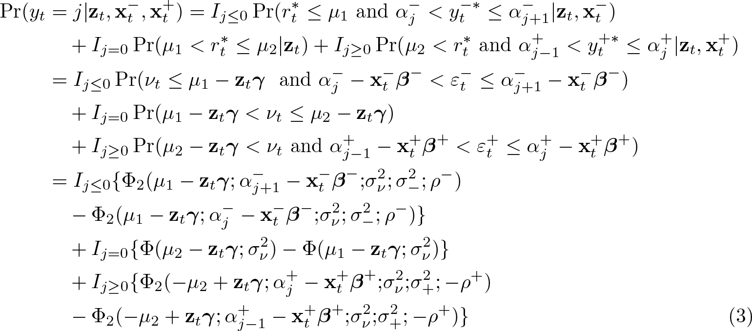
The probabilities of the outcome j in the NOP model are given by

\begin{matrix} \Pr (y_{t} = j ∣ z_{t}, x_{t}^{-}, x_{t}^{+}) = I_{j < 0} \Pr (r_{t}^{*} \leq μ_{1} and α_{j}^{-} < y_{t}^{- *} \leq α_{j + 1}^{-} ∣ z_{t}, x_{t}^{-}) \\ + I_{j = 0} \Pr (μ_{1} < r_{t}^{*} \leq μ_{2} ∣ z_{t}) + I_{j > 0} \Pr (μ_{2} < r_{t}^{*} and α_{j - 1}^{+} < y_{t}^{+ *} \leq α_{j}^{+} ∣ z_{t}, x_{t}^{+}) \\ = I_{j < 0} \Pr (ν_{t} \leq μ_{1} - z_{t} γ and α_{j}^{-} - x_{t}^{-} β^{-} < ε_{t}^{-} \leq α_{j + 1}^{-} - x_{t}^{-} β^{-}) \\ \begin{array}{l} + I_{j = 0} \Pr (μ_{1} - z_{t} γ < ν_{t} \leq μ_{2} - z_{t} γ) \\ + I_{j > 0} \Pr (μ_{2} - z_{t} γ < ν_{t} and α_{j - 1}^{+} - x_{t}^{+} β^{+} < ε_{t}^{+} \leq α_{j}^{+} - x_{t}^{+} β^{+}) \end{array} \\ \begin{matrix} = I_{j < 0} {Φ_{2} (μ_{1} - z_{t} γ; α_{j + 1}^{-} - x_{t}^{-} β^{-}; σ_{ν}^{2}; σ_{-}^{2}; ρ^{-}) \\ \begin{array}{l} - Φ_{2} (μ_{1} - z_{t} γ; α_{j}^{-} - x_{t}^{-} β -; σ_{ν}^{2}; σ_{-}^{2}; ρ^{-})} \\ + I_{j = 0} {Φ (μ_{2} - z_{t} γ; σ_{ν}^{2}) - Φ (μ_{1} - z_{t} γ; σ_{ν}^{2})} \\ + I_{j > 0} {Φ_{2} (- μ_{2} + z_{t} γ; α_{j}^{+} - x_{t}^{+} β^{+}; σ_{ν}^{2}; σ_{+}^{2}; - ρ^{+}) \\ - Φ_{2} (- μ_{2} + z_{t} γ; α_{j - 1}^{+} - x_{t}^{+} β^{+}; σ_{ν}^{2}; σ_{+}^{2}; - ρ^{+})} \end{array} \end{matrix} \end{matrix}

where I_j _< ₀ is an indicator function such that I_j _< ₀ = 1 if j < 0 and I_j _< ₀ = 0 if j ≥ 0 (analogously for I_j ₌₀ and I_j _> ₀).

In the case of exogenous switching (when ρ ⁻ = ρ ⁺ = 0), the probabilities of the outcome j in the NOP can be computed as

\begin{array}{l} \Pr (y_{t} = j ∣ z_{t}, x_{t}^{-}, x_{t}^{+}, ρ^{-} = ρ^{+} = 0) \\ = I_{j < 0} Φ (μ_{1} - z_{t} γ; σ_{ν}^{2}) {Φ (α_{j + 1}^{-} - x_{t}^{-} β^{-}; σ_{-}^{2}) - Φ (α_{j}^{-} - x_{t}^{-} β^{-}; σ_{-}^{2})} \\ + I_{j = 0} {Φ (μ_{2} - z_{t} γ) - Φ (μ_{1} - z_{t} γ)} \\ + I_{j > 0} {1 - Φ (μ_{2} - z_{t} γ; σ_{ν}^{2})} {Φ (α_{j}^{+} - x_{t}^{+} β^{+}; σ_{+}^{2}) - Φ (α_{j - 1}^{+} - x_{t}^{+} β^{+}; σ_{+}^{2})} \end{array}

In the case of two- or three-outcome choices, the NOP model degenerates to the conventional single-equation OP model.

2.3 Two-part zero-inflated ordered probit model

The two-part zero-inflated ordered probit (ZIOP-2) model, which represents the zero-inflated OP model of Brooks, Harris, and Spencer (2012) and the middle-inflated OP model of Bagozzi and Mukherjee (2012), can be described by the following system:

\begin{array}{l} Regime decision: & r_{t}^{*} = z_{t} γ + ν_{t} s_{t}^{*} = {\begin{matrix} 1 & if & μ < r_{t}^{*} \\ 0 & if & r_{t}^{*} \leq μ \end{matrix} \\ Outcome decision: & \begin{array}{l} y_{t}^{*} = x_{t} β + ε_{t} \\ y_{t} = {\begin{array}{l} j & if s_{t}^{*} = 1 and α_{j - 1} < y_{t}^{*} \leq α_{j} \\ 0 & if s_{t}^{*} = 0 \end{array} \\ where - \infty = α_{- J^{-} - 1} \leq α_{- J^{-}} \leq \dots \leq α_{J^{+}} = \infty \end{array} \\ Correlation among decisions: & [\begin{array}{l} ν_{t} \\ ε_{t} \end{array}] \overset{i.i.d.}{~} N (\begin{array}{l} 0 \\ 0 \end{array}, [\begin{matrix} σ_{ν}^{2} & ρ σ_{ν} σ \\ ρ σ_{ν} σ & σ^{2} \end{matrix}]) \end{array}

The probabilities of the outcome j in the ZIOP-2 model are given by

\begin{array}{l} \Pr (y_{t} = j ∣ z_{t}, x_{t}) = I_{j = 0} \Pr (r_{t}^{*} \leq μ ∣ z_{t}) + \Pr (μ < r_{t}^{*} and α_{j - 1} < y_{t}^{*} \leq α_{j} ∣ z_{t}, x_{t}) \\ = I_{j = 0} \Pr (ν_{t} \leq μ - z_{t} γ) + \Pr (μ - z_{t} γ < ν_{t} and α_{j - 1} - x_{t} β < ε_{t} \leq α_{j} - x_{t} β) \\ = I_{j = 0} Φ (μ - z_{t} γ; σ_{ν}^{2}) + Φ_{2} (- μ + z_{t} γ; α_{j} - x_{t} β; σ_{ν}^{2}; σ^{2}; - ρ) \\ - Φ_{2} (- μ + z_{t} γ; α_{j - 1} - x_{t} β; σ_{ν}^{2}; σ^{2}; - ρ) \end{array}

In the case of exogenous switching (when ρ = 0), these probabilities can be computed as follows:

\begin{matrix} \Pr (y_{t} = j ∣ z_{t}, x_{t}, ρ = 0) = I_{j = 0} Φ (μ - z_{t} γ; σ_{ν}^{2}) \\ + {1 - Φ (μ - z_{t} γ; σ_{ν}^{2})} \\ {Φ (α_{j} - x_{t} β; σ^{2}) - Φ (α_{j - 1} - x_{t} β; σ^{2})} \end{matrix}

If y_t ≥ 0 for ∀t, the ZIOP-2 model becomes the model of Harris and Zhao (2007).

2.4 Three-part zero-inflated ordered probit model

The three-part zero-inflated ordered probit (ZIOP-3) model developed by Sirchenko (2020) is a three-part generalization of the ZIOP-2 model and can be described by the following system:

\begin{array}{l} Regime decision: & r_{t}^{*} = z_{t} γ + ν_{t}, s_{t}^{*} = {\begin{matrix} 1 & if & μ_{2} < r_{t}^{*} \\ 0 & if & μ_{1} < r_{t}^{*} \leq μ_{2} \\ - 1 & if & r_{t}^{*} \leq μ_{1} \end{matrix} \\ Outcome decisions: & \begin{array}{l} y_{t}^{- *} = x_{t}^{-} β^{-} + ε_{t}^{-}, y_{t}^{+ *} = x_{t}^{+} β^{+} + ε_{t}^{+} \\ {\begin{array}{l} j & (j \geq 0) & if & s_{t}^{*} = 1 and α_{j - 1}^{+} < y_{t}^{+ *} \leq α_{j}^{+} \\ 0 & if & s_{t}^{*} = 0 \\ j & (j \leq 0) & if & s_{t}^{*} = - 1 and α_{j}^{-} < y_{t}^{- *} \leq α_{j + 1}^{-} \end{array} \\ \begin{array}{l} where - \infty = α_{- 1}^{+} \leq α_{0}^{+} \leq \dots \leq α_{J^{+}}^{+} = \infty \\ and - \infty = α_{- J^{-}}^{-} \leq α_{- J^{-} + 1}^{-} \leq \dots \leq α_{1}^{-} = \infty \end{array} \end{array} \\ Correlation among decisions: & [\begin{matrix} ν_{t} \\ ε_{t}^{i} \end{matrix}] \overset{i . i . d}{\sim} N (\begin{array}{l} 0 \\ 0 \end{array}, [\begin{matrix} σ_{ν}^{2} & ρ^{i} σ_{ν} σ_{i} \\ ρ^{i} σ_{ν} σ_{i} & σ_{i}^{2} \end{matrix}]), i \in {-, +} \end{array}

The probabilities of the outcome j in the ZIOP-3 model are given by

\begin{array}{l} \Pr (y_{t} = j ∣ z_{t}, x_{t}^{-}, x_{t}^{+}) = I_{j \leq 0} \Pr (r_{t}^{*} \leq μ_{1} and α_{j}^{-} < y_{t}^{- *} \leq α_{j + 1}^{-} ∣ z_{t}, x_{t}^{-}) \\ + I_{j = 0} \Pr (μ_{1} < r_{t}^{*} \leq μ_{2} ∣ z_{t}) + I_{j \geq 0} \Pr (μ_{2} < r_{t}^{*} and α_{j - 1}^{+} < y_{t}^{+ *} \leq α_{j}^{+} ∣ z_{t}, x_{t}^{+}) \\ = I_{j \leq 0} \Pr (ν_{t} \leq μ_{1} - z_{t} γ and α_{j}^{-} - x_{t}^{-} β^{-} < ε_{t}^{-} \leq α_{j + 1}^{-} - x_{t}^{-} β^{-}) \\ + I_{j = 0} \Pr (μ_{1} - z_{t} γ < ν_{t} \leq μ_{2} - z_{t} γ) \\ + I_{j \geq 0} \Pr (μ_{2} - z_{t} γ < ν_{t} and α_{j - 1}^{+} - x_{t}^{+} β^{+} < ε_{t}^{+} \leq α_{j}^{+} - x_{t}^{+} β^{+}) \\ = I_{j \leq 0} {Φ_{2} (μ_{1} - z_{t} γ; α_{j + 1}^{-} - x_{t}^{-} β^{-}; σ_{ν}^{2}; σ_{-}^{2}; ρ^{-}) \\ - Φ_{2} (μ_{1} - z_{t} γ; α_{j}^{-} - x_{t}^{-} β^{-}; σ_{ν}^{2}; σ_{-}^{2}; ρ^{-})} \\ + I_{j = 0} {Φ (μ_{2} - z_{t} γ; σ_{ν}^{2}) - Φ (μ_{1} - z_{t} γ; σ_{ν}^{2})} \\ + I_{j \geq 0} {Φ_{2} (- μ_{2} + z_{t} γ; α_{j}^{+} - x_{t}^{+} β^{+}; σ_{ν}^{2}; σ_{+}^{2}; - ρ^{+}) \\ - Φ_{2} (- μ_{2} + z_{t} γ; α_{j - 1}^{+} - x_{t}^{+} β^{+}; σ_{ν}^{2}; σ_{+}^{2}; - ρ^{+})} \end{array}

where I_j _≤ ₀ is an indicator function such that I_j _≤ ₀ = 1 if j ≤ 0 and I_j _≤ ₀ = 0 if j > 0 (analogously for I_j _≥ ₀).

In the case of exogenous switching (when ρ ⁻ = ρ ⁺ = 0), these probabilities can be computed as

\begin{array}{l} \Pr (y_{t} = j ∣ z_{t}, x_{t}^{-}, x_{t}^{+}, ρ^{-} = ρ^{+} = 0) = I_{j \leq 0} Φ (μ_{1} - z_{t} γ; σ_{ν}^{2}) {Φ (α_{j + 1}^{-} - x_{t}^{-} β^{-}; σ_{-}^{2}) \\ - Φ (α_{j}^{-} - x_{t}^{-} β^{-}; σ_{-}^{2})} + I_{j = 0} {Φ (μ_{2} - z_{t} γ; σ_{ν}^{2}) - Φ (μ_{1} - z_{t} γ; σ_{ν}^{2})} \\ + I_{j \geq 0} {1 - Φ (μ_{2} - z_{t} γ; σ_{ν}^{2})} {Φ (α_{j}^{+} - x_{t}^{+} β^{+}; σ_{+}^{2}) - Φ (α_{j - 1}^{+} - x_{t}^{+} β^{+}; σ_{+}^{2})} \end{array}

The inflated outcome does not have to be in the very middle of the ordered choices. If it is located at the end of the ordered scale—that is, if y_t ≥ 0 for ∀t—the ZIOP-3 model reduces to the ZIOP-2 model of Harris and Zhao (2007).

2.5 Maximum likelihood estimation

The probabilities in each OP equation can be consistently estimated under fairly general conditions by an asymptotically normal maximum likelihood (ML) estimator (Basu and de Jong 2007). The simultaneous estimation of the OP equations in the NOP, ZIOP-2, and ZIOP-3 models can also be performed using an ML estimator of the vector of the parameters θ that maximizes the log-likelihood function l( θ ):

\max_{θ ϵ Θ} l (θ) = \max_{θ ϵ Θ} \sum_{t = 1}^{T} \sum_{j = - J^{-}}^{J^{+}} I_{t j} \ln {\Pr (y_{t} = j ∣ x_{t}^{all}, θ)}

where I_tj is an indicator function such that I_tj = 1 if y_t = j and I_tj = 0 otherwise; θ includes γ , µ , β ⁻, β ⁺, α ⁻, α ⁺, ρ ⁻, and ρ ⁺ for the NOP and ZIOP-3 models, and includes γ , µ, β , α , and ρ for the ZIOP-2 model; Θ is a parameter space; $x_{t}^{all}$ is a vector that contains the values of all independent variables in the model; and $\Pr (y_{t} = j ∣ x_{t}^{all}, θ)$ are the probabilities from either (1) or (2) or (3). The asymptotic standard errors of $\hat{θ}$ can be computed from the Hessian matrix.

The intercept components of β , β ⁻, β ⁺, and γ are identified up to scale and location, that is, only jointly with the corresponding threshold parameters α , α ⁻, α ⁺, and µ and variances $σ^{2}, σ_{-}^{2}, σ_{+}^{2},$ and $σ_{ν}^{2}$ . As is common in the identification of discrete-choice models, the variances $σ^{2}, σ_{-}^{2}, σ_{+}^{2},$ and $σ_{ν}^{2}$ are fixed to 1, and the intercept components of β , β ⁻, β ⁺ and γ are fixed to 0. The probabilities in (1), (2), and (3) are invariant to these (arbitrary) identifying assumptions: up to scale and location, we can identify all parameters in θ because of the nonlinearity of OP equations, that is, via the functional form (Heckman 1978; Wilde 2000). However, because the normal CDF is approximately linear in the middle of its support, the simultaneous estimation of two or three equations may experience a weak identification problem if the regime and outcome equations contain the same set of independent variables. To enhance the precision of parameter estimates, we may impose exclusion restrictions on the specification of the independent variables in each equation.

The three regimes (nests) in the NOP model are fully observable, contrary to the latent (only partially observed) regimes in the ZIOP-2 and ZIOP-3 models. The likelihood function of the NOP model in the case of exogenous switching—again in contrast

with the ZIOP-2 and ZIOP-3 models—is separable with respect to the parameters in the three equations.² In the case of endogenous switching, the likelihood function in the ZIOP-2 and ZIOP-3 models, similar to the likelihood in mixture models, sample-selection models, and zero-inflated negative binomial models (Olsen 1982; Silva 2017), may have multiple local maximums. The ML estimates may depend on the starting values of the parameters; ideally, the initial values in the neighborhood of the global maximum can facilitate estimation.

To avoid the local maximums problem and to reduce computation costs, the following scanning procedure is implemented. The starting values for the slope and threshold parameters in the exogenous-switching models are obtained using the independent OP estimations of each equation. The starting values for ρ, ρ ⁻, and ρ ⁺ in the endogenous-switching models are obtained by maximizing the likelihood functions over a grid search from −0.95 to 0.95 in increments of 0.05, holding the other parameters fixed at their estimates in the corresponding exogenous-switching model. Olsen (1982) suggests a scanning procedure for ρ in the context of the sample-selection model and demonstrates that the likelihood function has a unique maximum for fixed values of ρ. To ensure that the maximum obtained is the global one, it make sense to try several starting points. The implemented estimators allow selecting any starting points. The Monte Carlo experiments confirm that the proposed estimators converge at the global maximum.

2.6 Marginal effects

We combine the marginal effects of each independent variable on the probability of each discrete outcome into a matrix ME _t , rows of which correspond to covariates and columns to outcomes. The marginal effects of continuous variable k (the kth element of x _t ^all) on the probability of outcome j are computed for the ZIOP-3 model as

\begin{matrix} M E_{k, j, t} = \frac{\partial \Pr (y_{t} = j ∣ θ)}{\partial x_{t, k}^{all}} = I_{j \leq 0} [{Φ (\frac{μ_{1} - z_{t} γ - ρ^{-} (α_{j}^{-} - x_{t}^{-} β^{-})}{\sqrt{1 - {(ρ^{-})}^{2}}}) f (α_{j}^{-} - x_{t}^{-} β^{-}) \\ - Φ (\frac{μ_{1} - z_{t} γ - ρ^{-} (α_{j + 1}^{-} - x_{t}^{-} β^{-})}{\sqrt{1 - {(ρ^{-})}^{2}}}) f (α_{j + 1}^{-} - x_{t}^{-} β^{-})} β_{k}^{- all} \\ - {Φ (\frac{α_{j + 1}^{-} - x_{t}^{-} β^{-} - ρ^{-} (μ_{1} - z_{t} γ)}{\sqrt{1 - {(ρ^{-})}^{2}}}) \\ - Φ (\frac{α_{j}^{-} - x_{t}^{-} β^{-} - ρ^{-} (μ_{1} - z_{t} γ)}{\sqrt{1 - {(ρ^{-})}^{2}}})} f (μ_{1} - z_{t} γ) γ_{k}^{all}] \\ \begin{array}{l} - I_{j = 0} {f (μ_{2} - z_{t} γ) - f (μ_{1} - z_{t} γ)} γ_{k}^{all} \\ + I_{j \geq 0} [{Φ (\frac{z_{t} γ ∣ - μ_{2} + ρ^{+} (α_{j - 1}^{+} - x_{t}^{+} β^{+})}{\sqrt{1 - {(ρ^{+})}^{2}}}) f (α_{j - 1}^{+} - x_{t}^{+} β^{+}) \end{array} \\ - Φ (\frac{z_{t} γ - μ_{2} + ρ^{+} (α_{j}^{+} - x_{t}^{+} β^{+})}{\sqrt{1 - {(ρ^{+})}^{2}}}) f (α_{j}^{+} - x_{t}^{+} β^{+})} β_{k}^{+ all} \\ + {Φ (\frac{α_{j}^{+} - x_{t}^{+} β^{+} + ρ^{+} (z_{t} γ - μ_{2})}{\sqrt{1 - {(ρ^{+})}^{2}}}) \\ - Φ (\frac{α_{j - 1}^{+} - x_{t}^{+} β^{+} + ρ^{+} (z_{t} γ - μ_{2})}{\sqrt{1 - {(ρ^{+})}^{2}}})} f (z_{t} γ - μ_{2}) γ_{k}^{all}] \end{matrix}

where f is the probability density function of the standard normal distribution, and $γ_{k}^{all}, β_{k}^{- all},$ and $β_{k}^{+ all}$ are the coefficients on the kth independent variable in $x_{t}^{all}$ in the regime equation, the outcome equation conditional on $s_{t}^{*} = 1,$ and the outcome equation conditional on $s_{t}^{*} = - 1,$ respectively ( $γ_{k}^{all}, β_{k}^{- all},$ or $β_{k}^{+ all}$ is 0 if the kth independent variable in $x_{t}^{all}$ is not included in the corresponding equation). For a discrete-valued independent variable, the ME can be computed as the change in the probabilities when this independent variable changes by one increment and all other variables are fixed.

The MEs for the NOP model are computed by replacing I_j _≥ ₀ in the above formula with I_j _> ₀ and I_j _≤ ₀ with I_j _< ₀.

The MEs for the ZIOP-2 model are computed as

\begin{matrix} {ME}_{k, j, t} = \frac{\partial \Pr (y_{t} = j ∣ θ)}{\partial x_{t, k}^{all}} = - I_{j = 0} {f (μ - z_{t} γ)} γ_{k}^{all} \\ + {Φ (\frac{z_{t} γ - μ + ρ (α_{j - 1} - x_{t} β)}{\sqrt{1 - ρ^{2}}}) f (α_{j - 1} - x_{t} β) \\ - Φ (\frac{z_{t} γ - μ + ρ (α_{j} - x_{t} β)}{\sqrt{1 - ρ^{2}}}) f (α_{j} - x_{t} β)} β_{k}^{all} \\ + {Φ (\frac{α_{j} - x_{t} β + ρ (z_{t} γ - μ)}{\sqrt{1 - ρ^{2}}}) \\ - Φ (\frac{α_{j - 1} - x_{t} β + ρ (z_{t} γ - μ)}{\sqrt{1 - ρ^{2}}})} f (z_{t} γ - μ) γ_{k}^{all} \end{matrix}

where $β_{k}^{all}$ is the coefficient on the kth independent variable in $x_{t}^{all}$ in the outcome equation ( $β_{k}^{all}$ is 0 if the kth independent variable in $x_{t}^{all}$ is not included in the outcome equation).

The asymptotic standard error of ME _k,j,t is computed using the delta method as a square root of $\nabla_{θ} (M E_{k, j, t}) V a r (θ) \nabla_{θ} (M {E^{'}}_{k, j, t}) .$

2.7 Relations among the models and their comparison

We now discuss the choice of a formal statistical test to compare the NOP, ZIOP-2, ZIOP-3, and conventional OP models. The choice depends on whether the models are nested in each other.

The exogenous-switching version of each model is nested in its endogenous-switching version as its uncorrelated special case; their comparison can be performed using any classical likelihood-based test for nested hypotheses, such as the likelihood-ratio (LR) test.

The OP is not nested either in the NOP or ZIOP-3 model. We can compare the OP model with them by using a likelihood-based test for nonnested models, such as the Vuong (1989) test.³ The OP model is, however, nested in the ZIOP-2 model. The latter reduces to the former if µ → −∞; hence, $\Pr (y_{t} = 0 ∣ x_{t}, s_{t}^{*} = 1) \to 0.$ Thus, the Vuong test for nonnested hypotheses cannot be used to compare the OP and ZIOP-2 models: for nested hypotheses, the Voung test reduces to the LR test. However, the critical values of the classical LR test are invalid in this case because some of the standard regularity conditions of the classical LR test fail to hold (Andrews 2001; Andrews and Cheng 2012). In particular, the value of µ in the null hypothesis is not an interior point of the parameter space; hence, the asymptotic distribution of the LR statistics is not standard.⁴

The NOP model is nested in the ZIOP-3 model. The latter becomes the former if $α_{- 1}^{-} \to \infty$ and $α_{1}^{+} \to - \infty$ ; therefore, $\Pr (y_{t} = 0 ∣ x_{t}^{+}, s_{t}^{*} = 1) \to 0$ and $\Pr (y_{t} = 0 ∣ x_{t}^{-}, s_{t}^{*} = - 1) \to 0.$ The values of $α_{- 1}^{-}$ and $α_{1}^{+}$ in the null hypothesis are not the interior points of the parameter space; thus, the asymptotic distribution of the LR statistics is not standard. The comparison of the NOP and ZIOP-3 models can also be performed using the LR test with simulated adjusted critical values (Andrews 2001; Andrews and Cheng 2012).

Generally, the ZIOP-2 model is not a special case of the ZIOP-3 model, and vice versa. We can compare them by using the Vuong test. A special case when the ZIOP-3 model nests the ZIOP-2 model emerges under certain restrictions on the parameters, as explained below. In this case, the selection between the ZIOP-3 and ZIOP-2 models can be performed using any classical likelihood-based test for nested hypotheses, such as the LR test.

The special case emerges if y_t takes on only three discrete values j ∊ {−1, 0, 1}, the regressors in $x_{t}^{-}$ and $x_{t}^{+}$ in the outcome equations of the ZIOP-3 model contain all the regressors in the ZIOP-2 regime equation (denoted below by z ₂ _t with the parameter vector γ ₂), and the regressors in the regime equation of the ZIOP-3 model (denoted below by z ₃ _t with the parameter vector γ ₃) include all the regressors in the x _t in the ZIOP-2 outcome equation. According to (2), the probabilities of the outcome j in the ZIOP-2 model are given by

\begin{array}{l} \Pr (y_{t} = - 1 ∣ z_{2 t}, x_{t}) = Φ_{2} (- μ + z_{2 t} γ_{2}; α_{- 1} - x_{t} β; - ρ) \\ \Pr (y_{t} = 0 ∣ z_{2 t}, x_{t}) = Φ (μ - z_{2 t} γ_{2}) + Φ_{2} (- μ + z_{2 t} γ_{2}; α_{0} - x_{t} β; - ρ) \\ - Φ_{2} (- μ + z_{2 t} γ_{2}; α_{- 1} - x_{t} β; - ρ) = 1 - Φ_{2} (- μ + z_{2 t} γ_{2}; - α_{0} + x_{t} β; ρ) \\ - Φ_{2} (- μ + z_{2 t} γ_{2}; α_{- 1} - x_{t} β; - ρ); \\ \Pr (y_{t} = 1 ∣ z_{2 t}, x_{t}) = Φ (- μ + z_{2 t} γ) - Φ_{2} (- μ + z_{2 t} γ_{2}; α_{0} - x_{t} β; - ρ) \\ = Φ_{2} (- μ + z_{2 t} γ_{2}; - α_{0} + x_{t} β; ρ) \end{array}

because $Φ_{2} (x; y; ρ) = Φ (x) − Φ_{2} (x;− y;− ρ)$ .

Similarly, according to (3) the probabilities of the outcome j in the ZIOP-3 model are given by

\begin{array}{l} \Pr (y_{t} = - 1 ∣ z_{3 t}, x_{t}^{-}, x_{t}^{+}) = Φ_{2} (μ_{1} - z_{3 t} γ_{3}; α_{0}^{-} - x_{t}^{-} β^{-}; ρ^{-}) \\ \Pr (y_{t} = 0 ∣ z_{3 t}, x_{t}^{-}, x_{t}^{+}) = Φ (μ_{1} - z_{3 t} γ_{3}) - Φ_{2} (μ_{1} - z_{3 t} γ_{3}; α_{0}^{-} - x_{t}^{-} β^{-}; ρ^{-}) \\ + Φ (μ_{2} - z_{3 t} γ_{3}) - Φ (μ_{1} - z_{3 t} γ_{3}) + Φ_{2} (- μ_{2} + z_{3 t} γ_{3}; α_{0}^{+} - x_{t}^{+} β^{+}; - ρ^{+}) \\ = Φ_{2} (μ_{1} - z_{3 t} γ_{3}; - α_{0}^{-} + x_{t}^{-} β^{-}; - ρ^{-}) + Φ (μ_{2} - z_{3 t} γ_{3}) \\ - Φ (μ_{1} - z_{3 t} γ_{3}) + Φ_{2} (- μ_{2} + z_{3 t} γ_{3}; α_{0}^{+} - x_{t}^{+} β^{+}; - ρ^{+}) \\ \Pr (y_{t} = 1 ∣ z_{3 t}, x_{t}^{-}, x_{t}^{+}) = Φ (- μ_{2} + z_{3 t} γ_{3}) - Φ_{2} (- μ_{2} + z_{3 t} γ_{3}; α_{0}^{+} - x_{t}^{+} β^{+}; - ρ^{+}) \\ = Φ_{2} (- μ_{2} ∣ + z_{3 t} γ_{3}; - α_{0}^{+} + x_{t}^{+} β^{+}; ρ^{+}) \end{array}

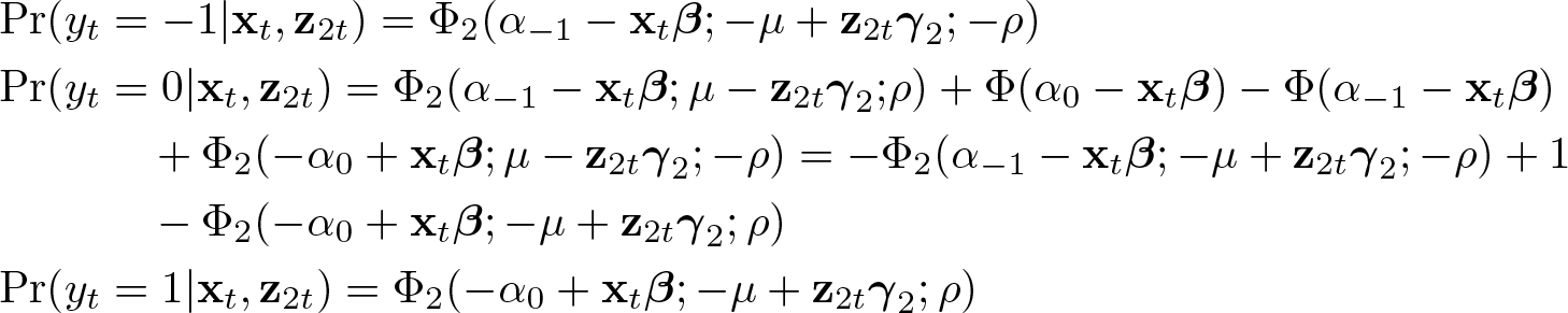
Suppose the regressors in $x_{t}^{-}$ and $x_{t}^{+}$ in the ZIOP-3 outcome equations are identical to the regressors in z ₂ _t in the ZIOP-2 regime equation, the regressors in z ₃ _t in the ZIOP-3 regime equation are identical to the regressors in the x _t in the ZIOP-2 outcome equation, and the parameters are restricted as follows: − β ⁻ = β ⁺ = γ ₂, β = γ ₃, µ ₁ = α ₋ ₁, $μ_{2} = α_{0}, - α_{0}^{-} = α_{0}^{+} = μ,$ and −ρ ⁻ = ρ ⁺ = ρ. Then, because $x_{t}^{-} = x_{t}^{+} = z_{2 t}, z_{3 t} = x_{t}$ and Φ(−x) = 1 − Φ(x), the probabilities for the ZIOP-3 model can be written as

\begin{array}{l} \Pr (y_{t} = - 1 ∣ x_{t}, z_{2 t}) = Φ_{2} (α_{- 1} - x_{t} β; - μ + z_{2 t} γ_{2}; - ρ) \\ \Pr (y_{t} = 0 ∣ x_{t}, z_{2 t}) = Φ_{2} (α_{- 1} - x_{t} β; μ - z_{2 t} γ_{2}; ρ) + Φ (α_{0} - x_{t} β) - Φ (α_{- 1} - x_{t} β) \\ + Φ_{2} (- α_{0} + x_{t} β; μ - z_{2 t} γ_{2}; - ρ) = - Φ_{2} (α_{- 1} - x_{t} β; - μ + z_{2 t} γ_{2}; - ρ) + 1 \\ - Φ_{2} (- α_{0} + x_{t} β; - μ + z_{2 t} γ_{2}; ρ) \\ \Pr (y_{t} = 1 ∣ x_{t}, z_{2 t}) = Φ_{2} (- α_{0} + x_{t} β; - μ + z_{2 t} γ_{2}; ρ) \end{array}

which are identical to the probabilities for the ZIOP-2 model in (5).

Notice that the restrictions − β ⁻ = β ⁺ = γ ₂ and $- α_{0}^{-} = α_{0}^{+} = μ$ impose a sort of symmetry in the ZIOP-3 model, because they imply that the conditional probability of a positive response is equal to the conditional probability of a negative response:

\begin{array}{l} \Pr (y_{t} = 1 ∣ z_{3 t}, x_{t}^{+}, s_{t}^{*} = 1) = 1 - Φ (α_{0}^{+} - x_{t}^{+} β^{+}) \\ = Φ (- α_{0}^{+} + x_{t}^{+} β^{+}) = Φ (α_{0}^{-} - x_{t}^{-} β^{-}) = \Pr (y_{t} = - 1 ∣ z_{t}, x_{t}^{-}, s_{t}^{*} = - 1) \end{array}

In general, if $x_{t}^{-}$ and $x_{t}^{+}$ are not identical to z ₂ _t but contain all the regressors in z ₂ _t , and if z ₃ _t is not identical to x _t but contains all the regressors in x _t , the ZIOP-2 model is still nested in the ZIOP-3 model with the additional zero restrictions for the coefficients on all the extra regressors in $x_{t}^{-}, x_{t}^{+},$ and z ₃ _t .

3 The nop, ziop2, and ziop3 commands

The accompanying software includes the three new commands, the postestimation commands, and the supporting help files.

3.1 Syntax

The following commands fit, respectively, the NOP, ZIOP-2, and ZIOP-3 models for discrete ordinal outcomes:

nop depvar indepvars [ if ] [ in ] [ , posindepvars( varlist ) negindepvars( varlist )

infcat( choice ) endoswitch robust cluster( varname ) vuong initial( string )

nolog]

ziop2 depvar indepvars [ if ] [ in ] [ , outindepvars( varlist ) infcat( choice )

endoswitch robust cluster( varname ) initial( string ) nolog]

ziop3 depvar indepvars [ if ] [ in ] [ , posindepvars( varlist )

negindepvars( varlist ) infcat( choice ) endoswitch robust cluster( varname )

vuong initial( string ) nolog ]

An ordinal dependent variable, depvar, is assumed to take on at least five discrete ordinal values in the NOP model, at least two in the ZIOP-2 model, and at least three in the ZIOP-3 model. A list of the independent variables in the regime equation, indepvars, may be different from the lists of the independent variables in the outcome equations.

Options

posindepvars( varlist ) specifies a list of the independent variables in the outcome equation, conditional on the regime $s_{t}^{*} = 1$ for nonnegative outcomes in the NOP and ZIOP-3 models. By default, it is identical to indepvars, the list of the independent variables in the regime equation.

negindepvars( varlist ) specifies a list of the independent variables in the outcome equation, conditional on the regime $s_{t}^{*} = - 1$ for nonpositive outcomes in the NOP and ZIOP-3 models. By default, it is identical to indepvars, the list of the independent variables in the regime equation.

outindepvars( varlist ) specifies a list of the independent variables in the outcome equation of the ZIOP-2 model. By default, it is identical to indepvars, the list of the independent variables in the regime equation.

infcat( choice ) is the value of the dependent variable in the regime $s_{t}^{*} = 0$ that should be modeled as inflated in the ZIOP-2 and ZIOP-3 models and modeled as neutral in the NOP model. The default is infcat(0).

endoswitch specifies that endogenous regime switching be used instead of default exogenous switching. Regime switching is endogenous if the unobserved random term in the regime equation is correlated with the unobserved random terms in the outcome equations; it is exogenous otherwise.

robust specifies that a robust sandwich estimator of variance be used; the default estimator is based on the observed information matrix.

cluster( varname ) specifies a clustering variable for the clustered robust sandwich estimator of variance.

vuong specifies that the Vuong test of the NOP (or ZIOP-3) model versus the conventional OP model be performed. The reported Vuong test statistics⁵ have a standard normal distribution with large positive values favoring the NOP (or ZIOP-3) model and large negative values favoring the OP model.

initial( string ) specifies a space-delimited list, string, of the starting values of the parameters in the following order: γ , µ , β ⁺, α ⁺, β ⁻, α ⁻, ρ ⁻, and ρ ⁺ for the NOP and ZIOP-3 models, and γ , µ, β , α , and ρ for the ZIOP-2 model.

nolog suppresses the iteration log and preliminary results.

Stored results

The descriptions of the stored results can be found in the help files.

3.2 Postestimation commands

The following postestimation commands are available after nop, ziop2, and ziop3:

The predict command

predict newvar [ if ] [ in ] [ , zeros regimes output( string ) ]

This command computes the predicted probabilities of the discrete choices (by default), the regimes and the types of zeros conditional on the regime, and the predicted outcomes and the expected values of the dependent variable for all observed values of the independent variables in the sample. The command creates (J ⁻ + J ⁺ + 1) new variables under the names with a newvar prefix. The following options are available:

zeros indicates that the probabilities of the different types of zeros (the outcomes in the inflated category infcat( choice ) in the ZIOP-2 and ZIOP-3 models), conditional on different regimes, be predicted instead of the choice probabilities.

regimes indicates that the probabilities of the regimes s_t ∊ {−1, 0, 1} be predicted instead of the choice probabilities. This option is ignored if the zeros option is used.

output( string ) specifies the different types of predictions. The possible values of string are as follows: choice for reporting the predicted outcome (the choice with the largest predicted probability); mean for reporting the expected value of the dependent variable computed as ∑ _i i Pr(y_t = i); and cum for predicting the cumulative choice probabilities, Pr(y_t ≤ −J ⁻), Pr(y_t ≤ −J ⁻ + 1),…, Pr(y_t ≤ J ⁺). By default, the usual choice probabilities, Pr(y_t = −J ⁻), Pr(y_t = −J ⁻ + 1),…, Pr(y_t = J ⁺), are predicted and saved into the new variables with the newvar prefix.

The ziopprobabilities command

ziopprobabilities [ , at( string ) zeros regimes ]

This command shows the predicted probabilities estimated at the specified values of the independent variables along with the standard errors. The options zeros and regimes are specified as in predict. The option at() is specified as follows:

at( string ) specifies for which values of the independent variables to estimate the predictions. string is a list of varname = value expressions, separated by commas. If at( string ) is used, the predictions are estimated at these values and displayed without saving to the dataset. If some independent variable names are not specified, their median values are taken instead. By default, the predictions are estimated at the median values of the independent variables.

The ziopcontrasts command

ziopcontrasts [ , at( string ) to( string ) zeros regimes ]

This command shows the differences in the predicted probabilities, estimated first at the values of the independent variables in at() and then at the values in to(), along with the standard errors. The options zeros, regimes, and at() are specified as in ziopprobabilities. The option to() is specified analogously to at().

The ziopmargins command

ziopmargins [ , at( string ) zeros regimes ]

This command shows the marginal effects of each independent variable on the predicted probabilities estimated at the specified values of the independent variables, along with the standard errors. The options zeros, regimes, and at() are specified as in ziopprobabilities.

The ziopclassification command

ziopclassification [ if ] [ in ]

This command shows the classification table (or confusion matrix); the percentage of correct predictions; the two strictly proper scores—the probability, or Brier, score (Brier 1950) and the ranked probability score (Epstein 1969); and the precisions, hit rates (or recalls), and adjusted noise-to-signal ratios (Kaminsky and Reinhart 1999).

The classification table reports the predicted choices (the ones with the highest predicted probability) in columns, the actual choices in rows, and the number of (mis)classifications in each cell.

The Brier probability score is computed as $1 / T \sum_{t = 1}^{T} \sum_{j = - J^{-}}^{J^{+}} {\Pr (y_{t} = j) - I_{j t}}^{2},$ where indicator I_jt = 1 if y_t = j and I_jt = 0 otherwise. The ranked probability score is computed as $1 / T \sum_{t = 1}^{T} \sum_{j = - J^{-}}^{J^{+}} {(Q_{j t} - D_{j t})}^{2},$ where $Q_{i t} = \sum_{i = - J^{-}}^{j} \Pr (y_{t} = i)$ and $D_{i t} = \sum_{i = - J^{-}}^{j} I_{j t} .$ The better the prediction, the smaller are both score values. Both scores have a minimum value of 0 when all the actual outcomes are predicted with a unit probability.

The precision, hit rate (or recall), and adjusted noise-to-signal ratios are defined as follows. Let TP denote a true positive event, that is, the outcome was predicted and occurred; let FP denote a false positive event, that is, the outcome was predicted but did not occur; let FN denote a false negative event, that is, the outcome was not predicted but did occur; and let TN denote a true negative event, that is, the outcome was not predicted and did not occur. The desirable outcomes fall into categories TP and TN, while the noisy ones fall into categories FP and FN. A perfect prediction has no entries in FP and FN, while a noisy prediction has many entries in FP and FN but few in TP and TN. The precision is defined for each choice as TP/(TP + FP); the recall is defined as TP/(TP + FN); and the adjusted noise-to-signal ratio is defined as {FP/(FP + TN)}/{TP/(TP + FN)}.

The ziopvuong command

ziopvuong modelspec ₁ modelspec ₂

This command performs the Vuong test for nonnested hypotheses, which compares the closeness of two models to the true data distribution by using the differences in the pointwise log likelihoods of the two models. The null hypothesis is that both models are misspecified but equally close to the unknown true model. The test statistic is equal to the average difference of the pointwise log likelihoods divided by the estimated standard error of those pointwise differences. Under the null hypothesis, the Vuong test statistic converges in distribution to a standard normal one. The arguments modelspec ₁ and modelspec ₂ are the names under which the estimation results are saved using the estimates store command. Any model that stores the vector e(ll_obs) of observationwise log likelihood can technically be used to perform the test. The command provides the three Vuong test statistics (z scores): the standard one and two adjusted ones with corrections to address the comparison of models with different numbers of parameters based on AIC and BIC. They can be used to test the hypothesis that one of the models explains the data better than the other. A significant positive z score indicates a preference for the first model, while a significant negative z score indicates a preference for the second model. An insignificant z score implies no preference for either model.

4 Monte Carlo experiments

We performed three sets of Monte Carlo simulations to illustrate the finite-sample performance of the ML estimators of each model. In the first set of experiments, we studied the performance of the ML estimators of the NOP, ZIOP-2, and ZIOP-3 models when simulated and estimated processes are the same, using artificial explanatory variables. The simulations demonstrate that the proposed ML estimators deliver consistent and reliable estimates even in small samples.

In the second set of experiments, using the real-world values of explanatory variables and the values of parameters from the empirical example, we compared the performance of the ML estimators of the OP and ZIOP-3 models if the data are generated by one of them and then fit by both models, and the performance of various measures of fit, information criteria, and statistical tests in selecting the best model. The ZIOP-3 estimator under the OP data-generating process (DGP) performs substantially better than the OP estimator under the ZIOP-3 DGP, and it produces reliable inference in small samples under both DGPs. AIC and BIC outperform the other criteria and tests in correctly selecting the true model under both DGPs.

In the third set of experiments, we compared the performance of the asymptotic and nonparametric bootstrap estimators of the standard errors. The simulations suggest that, in small samples, the bootstrap estimator of the standard errors of the parameters in the models with endogenous switching may provide substantially better coverage rates than the asymptotic estimator, especially with regard to the correlation coefficients. However, the bootstrap estimator of the standard errors of the choice probabilities does not necessarily perform better than the asymptotic one at the same time.

4.1 Monte Carlo design

In the first set of experiments, we simulated six DGPs according to the NOP, ZIOP-2, and ZIOP-3 models (each of them with both exogenous and endogenous switching) and then estimated each process by using the true model. Three independent variables, w₁ , w₂ , and w₃ , were drawn in each replication as $w_{1} \overset{i.i.d.}{\sim} N (0, 1) + 2, w_{2} \overset{i.i.d.}{\sim} N (0, 1),$ and w₃ = −1 if u ≤ 0.3, 0 if 0.3 < u ≤ 0.7, or 1 if u > 0.7, where $u \overset{i.i.d.}{\sim} U [0, 1]$ . The repeated samples were generated for the NOP and ZIOP-3 models with Z = (w₁ , w₂ ), X ⁻ = (w₁ , w₃ ), X ⁺ = (w₂ , w₃ ), and for the ZIOP-2 model with Z = (w ₁, w ₃), X = (w ₂, w ₃). The dependent variable y was generated with five values: −2, −1, 0, 1, and 2. The parameters were calibrated to yield, on average, the following frequencies of the above outcomes: 7%, 14%, 58%, 14%, and 7%, respectively. The true values of parameters in the simulations, θ _true, are shown in table A1 in the appendix. Ten thousand repeated samples with T = 200, 500, and 1,000 observations were independently generated for each DGP.

In the second set of experiments, we simulated two DGPs. One is generated by the OP model, and the other is generated by the ZIOP-3 model with exogenous switching. For each DGP, we fit both models. We simulated data by mimicking the real-world sample used in our empirical application in section 5. The values of four regressors (spread, pb, houst, and gdp) were the same as in the empirical example and held fixed in all replications. The standard normal error terms were independently drawn in each replication. The values of the dependent variable (−2, −1, 0, 1, or 2) were generated according to the OP and ZIOP-3 models using the same specifications and the same values of the parameters as in the estimations reported in section 5. Ten thousand repeated samples with 210 observations were independently generated for each DGP.

In the third set of experiments, we simulated four DGPs according to the NOP and ZIOP-3 models (each of them with both exogenous and endogenous switching), as in the first set of experiments, and we estimated each process using the true model and using both the asymptotic and the bootstrap estimators of the standard errors. We generated 3,000 replications in the case of exogenous switching and 1,000 replications in the case of endogenous switching. To compute a nonparametric bootstrap estimator of standard errors, we drew with replacement 200 bootstrap samples for each Monte Carlo iteration, recalculated the statistics, and obtained the standard deviations of the replicated statistics.

To avoid the divergence of the ML estimates due to the problem of complete separation (perfect prediction), which could happen if the actual number of observations in any outcome category is 0 or very low, the samples with any outcome category frequency lower than 6% (in the first and third sets of experiments), 4% (in the second set), and 3% (in the bootstrap samples) were discarded. The variances of the normal error terms in all experiments were fixed to 1.

4.2 Monte Carlo results

Table 1 reports the measures of accuracy for the ML estimates of the slope parameters β , β ⁻, β ⁺, and γ and correlation coefficients ρ, ρ ⁻, and ρ ⁺ in the first set of experiments. The simulations show that the estimators are consistent: as sample size increases from 200 to 1,000, the biases decrease at least fourfold and the root mean squared errors (RMSE) decrease at least twice. The coverage rate for the slope parameters is below 90% only for the ZIOP-3 model with 200 observations; for the other sample sizes and models, the coverage rates are between 91.1% and 95.1%; with 1,000 observations, the biases of the standard error estimates are smaller than 5% and the coverage rates are between 93.4% and 95.1%. The coverage rates for the correlation coefficients are not so good: between 68% and 79% with 200 observations and between 82% and 93% with 1,000 observations.

Table 1.

The accuracy of the estimators of parameters

Sample size	True and fit model	NOP (ρ ⁻ = ρ ⁺ = 0)	NOP	ZIOP-2 (ρ = 0)	ZIOP-2	ZIOP-3 (ρ ⁻ = ρ ⁺ = 0)	ZIOP-3
Slope coefficients β , β ⁻, β ⁺, and γ
200	Bias, ×100	4.5	2.5	20.2	8.4	4.9	5.0
500		1.5	1.0	3.5	2.9	2.2	3.1
1000		0.8	0.5	1.5	1.2	1.1	1.2
200	RMSE, ×10	4.6	7.9	21.6	3.8	2.6	2.6
500		1.4	1.4	1.8	1.7	1.5	1.5
1000		0.9	1.0	1.1	1.0	1.0	1.0
200	Coverage rate (at 95% level), %	95.1	92.4	91.2	91.1	92.1	88.3
500		94.9	93.2	93.4	93.4	92.8	91.4
1000		95.1	93.9	94.6	94.8	93.5	93.4
200	Bias of standard error estimates, %	18.2	12.0	48.1	20.8	13.8	12.6
500		3.0	2.3	12.6	8.3	6.6	5.9
1000		1.1	1.9	3.3	2.7	4.1	2.7
Correlation coefficients ρ, ρ ⁻, and ρ ⁺
200	Bias		0.10		0.05		0.25
500			0.04		0.01		0.08
1000			0.02		0.01		0.03
200	RMSE, ×10		5.1		4.1		6.1
500			3.4		2.4		4.2
1000			2.5		1.6		3.1
200	Coverage rate (at 95% level), %		68.8		78.7		73.8
500			76.8		87.0		80.3
1000			82.6		92.6		85.1
200	Bias of standard error estimates, %		16.0		18.4		6.2
500			13.7		5.6		8.2
1000			10.0		2.9		7.4

notes: Bias is the absolute difference between the estimated and true values (in case of standard error estimates, divided by the true value; the true value is computed as the standard deviation of the estimates in all replications). RMSE is the root mean squared error of the estimates. Coverage rate is the percentage of times the estimated asymptotic 95% confidence intervals cover the true values. The above measures are averaged across all parameters.

Table 2 reports the measures of accuracy of the estimates of choice probabilities. The accuracy of estimated probabilities is more interesting and informative than the accuracy of estimated parameters. In the latent class models, the parameters are identified only up to scale and location and cannot be easily interpreted in terms of ME on the probabilities (for example, in the OP models, the sign of the coefficient on a certain covariate does not imply the direction of the ME of that covariate). In contrast, the choice probabilities are absolutely estimable and invariant to the identifying assumptions, which are necessary to estimate the latent class models. The estimates of the choice probabilities are the primary objectives of empirical studies. Besides, the percent bias of parameter estimates in simulations depends on the chosen absolute values of the parameters, whereas the percent bias of probability estimates is invariant to them.

Table 2.

The accuracy of the estimators of choice probabilities

Sample size	True and fit model	NOP (ρ ⁻ = ρ ⁺ = 0)	NOP	ZIOP-2 (ρ = 0)	ZIOP-2	ZIOP-3 (ρ ⁻ = ρ ⁺ = 0)	ZIOP-3
200	Bias, ×1000	1.8	1.9	4.8	6.1	4.1	4.9
500		0.8	1.0	2.4	3.4	2.0	2.8
1000		0.4	0.5	1.4	1.9	0.9	1.7
200	RMSE, ×100	2.4	2.6	2.8	2.9	2.7	2.9
500		1.5	1.6	1.7	1.8	1.6	1.8
1000		1.1	1.1	1.2	1.2	1.1	1.3
200	Coverage rate (at 95% level), %	94.4	94.4	95.3	95.3	95.1	94.8
500		95.4	95.2	95.6	95.6	95.9	95.7
1000		95.5	95.5	95.7	95.7	95.6	95.6
200	Bias of standard error estimates, %	4.2	4.2	6.9	6.4	5.5	15.1
500		3.9	4.6	6.9	6.1	5.3	16.6
1000		2.6	3.4	5.7	5.9	3.7	13.9

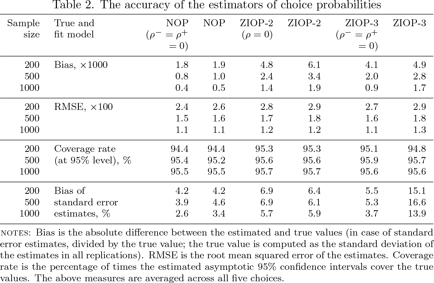
The values of the choice probabilities, which depend on the values of the regressors, are computed for table 2 at the population means of the simulated regressors. The probability estimates are more accurate than the parameter estimates. The simulations show that the ML estimates of probabilities are consistent and reliable even in samples with only 200 observations: the biases are smaller than five percent and the asymptotic coverage rates differ from the nominal 0.95 level by less than 1%. With 1,000 observations, the biases of choice probability estimates are around 1%. For each model, the biases and RMSE sharply decrease as the sample size increases from 200 to 1,000. The RMSE decreases, in most cases, faster than the asymptotic rate $\sqrt{T}$ . This may be caused by a small number of large deviations in the parameter estimates in small samples. For all models and sample sizes, the biases and RMSE are, as expected, slightly higher in more complex endogenous-switching versions. The standard error estimates, on average, correspond to the actual standard errors; however, large deviations make standard error estimates biased in small samples, but do not move the coverage rates from the nominal level by more than 1% even with only 200 observations. The accuracy in the NOP models is, as expected, higher than in the zero-inflated OP models.

Table 3 reports the results of the second set of experiments. To compare the performance of the OP and ZIOP-3 models fit under each DGP, the two top panels of table 3 show for both fitted models the accuracy of the estimated probability of the actual (observed) choice and the accuracy of the estimated ME of the regressor spread on the probability of the actual choice. The probabilities and MEs are computed at the actual values of the regressors for all observations in the repeated samples and averaged across all observations and all samples. The OP model under the ZIOP-3 DGP performs substantially worse than the ZIOP-3 model under the OP DGP. The biases in the OP model under the ZIOP-3 DGP are 3 times (for probability) and 18 times (for ME) as large as the biases in the ZIOP-3 model, whereas the biases in the ZIOP-3 model under the OP DGP are similar to the biases in the true model. The differences in the RMSE in two models under each DGP are comparable. The ZIOP-3 model clearly outperforms the OP model in terms of the coverage rates: the estimated asymptotic 95% confidence intervals in the ZIOP-3 model cover the true values in about 90% of iterated samples under both DGPs, while the coverage rate of the OP model is around 94% under its own DGP but around 54% only under the ZIOP-3 DGP.

Table 3.

The performance of the OP and ZIOP-3 models under each DGP

True model	OP		ZIOP-3
Fit model	OP	ZIOP-3	OP	ZIOP-3
Estimated probability of actual choice
Bias, ×100	0.8	1.0	−4.9	1.6
RMSE, ×100	6.4	10.2	17.2	9.0
Coverage rate, %	93.6	88.2	54.0	88.7
Estimated marginal effect of spread on probability of actual choice
Bias, ×100	−0.5	−0.4	−3.6	−0.2
RMSE, ×100	10.2	17.1	23.4	21.2
Coverage rate, %	94.6	89.1	53.9	91.3
Model selection results (fraction of times when a model is selected according to each criterion)
% of correct predictions	0.45	0.46	0.02	0.96
Brier score	0.50	0.50	0.00	1.00
Ranked probability score	0.55	0.45	0.00	1.00
LR test	0.53	0.47	0.00	1.00
AIC	0.96	0.04	0.00	1.00
BIC	1.00	0.00	0.05	0.95
Vuong test	0.05	0.02	0.00	1.00
Vuong test (AIC)	0.56	0.00	0.00	0.96
Vuong test (BIC)	0.99	0.00	0.00	0.54
Sign test	0.13	0.26	0.00	1.00
Sign test (AIC)	0.84	0.01	0.01	0.96
Sign test (BIC)	1.00	0.00	0.12	0.41

notes: Bias is the difference between the estimated and true values, multiplied by 100. RMSE is the root mean squared error of the estimates, multiplied by 100. Coverage rate is the percentage of times the estimated asymptotic 95% confidence intervals cover the true values. The probabilities and MEs are computed at the actual values of regressors for all observations.

The bottom panel of table 3 shows the fractions of times when a model is selected under each DGP according to the following measures of fit, information criteria, and statistical tests: the percentage of correct predictions (according to a maximum probability rule), the Brier score, the ranked probability score, the LR test, the information-based selection criteria AIC and BIC, the Vuong tests, and the pared sign tests (Clarke 2003). Information criteria are computed as AIC = −2l( θ _ML)+2p and BIC = −2l( θ _ML)+p(lnT), where p is the total number of estimated parameters and l( θ _ML) is the maximized log-likelihood function. To perform the sign test, we computed the differences of the pointwise log likelihoods of two models and counted the number of positive differences. Under the null hypothesis that both models are equally distant from the true model, half of the log-likelihood ratios should be positive and half should be negative. Under the null, the number of positive differences is distributed binomial (with 0.5 probability of success in each of T = 210 trials). The Vuong and pared sign tests are performed in the classical form as well as with the Akaike and Bayesian penalties [respectively, p/T and p(lnT)/(2T)] for the pointwise log likelihoods.

The model selection results demonstrate the superiority of the ZIOP-3 model and back the need for its zero-inflation component. Under its own DGP, the ZIOP-3 model is selected in 95%–100% of cases by all criteria except for the Vuong test with Bayesian penalty (54% of cases) and sign test with Bayesian penalty (41%), while the OP model is never selected by any criteria except for the percentage of correct predictions (in 2% of cases only), BIC (5% only), and sign tests with Akaike (1% only) and Bayesian (12% only) penalties. In contrast, under the OP DGP, the selection results are not so overwhelmingly in favor of the true model: the OP model is preferred in 96%–100% of cases by AIC, BIC, and the Vuong and sign tests with Bayesian penalty, but in 5% of cases only by the Vuong test, in 13% of cases only by the sign test, and in 84% of cases by the sign test with Akaike penalty; the other tests and criteria select the true OP model in 45%–56% of cases only. The ZIOP-3 model is selected under the OP DGP far more often than the OP model under the ZIOP-3 DGP. Under the OP DGP, the ZIOP-3 model is even more often preferred by the sign test (in 26% of cases) than the true model (in 13% of cases only).

BIC and AIC do the best job correctly selecting the true model in at least 95% of cases under both DGPs. Under the zero-inflated DGP, when the ZIOP-3 model clearly outperforms the OP model, most of the criteria perform well and correctly favor the true model in at least 95% of cases except for the Vuong and sign tests with Bayesian penalty: the former selects the true model in 54% of cases only but never selects the OP model, while the latter selects the ZIOP-3 model in 42% of cases but prefers the OP model in 12% of cases. Under the OP DGP, when the performance of the ZIOP-3 model is quite close to that of the OP model, only AIC, BIC, and the Vuong and sign tests with Bayesian penalties perform well and correctly select the true model in more than 95% of cases. The classical LR/Vuong/sign tests select the true model only in 53%/5%/13% of cases, prefer the wrong model in 47%/2%/26% of cases, and are indifferent between the two alternatives in 0%/93%/61% of cases. Such criteria as the percentage of correct predictions, the Brier score, and the ranked probability score, which are not based on the ML approach, select each alternative in roughly one half of cases, though the ranked probability score performs slightly better than the others, selecting the true model in 55% of cases.

Table 4 summarizes the results of the third set of experiments. As the upper panel shows, the asymptotic estimates of the standard errors of the slope parameters are rather slightly underestimated (by 9%–13%), whereas the bootstrap estimates are severely overestimated (by 155%–325% for exogenous switching and by 16%–22% for endogenous switching). The more complicated the model, the worse (the lower) are the asymptotic coverage rates: 95% for the NOP with exogenous switching, but only 86% for the ZIOP-3 with endogenous switching. The bootstrap coverage rates are above the 95% nominal level (in the 96.6%–98.4% interval); they are closer to the nominal level than the asymptotic ones for both models with endogenous switching, have the same deviation from the nominal level (but in the opposite directions) for the ZIOP-3 model with exogenous switching, and are further from the nominal level for the NOP model with exogenous switching.

Table 4.

Comparison of the asymptotic and bootstrap estimators of standard errors

True and fit model		NOP (ρ ⁻ = ρ ⁺ = 0)	NOP	ZIOP-3 (ρ ⁻ = ρ ⁺ = 0)	ZIOP-3
Slope coefficients β ⁻, β ⁺, and γ
Coverage rate	Asymptotic	95.0	93.0	91.9	86.2
(at 95% level), %	Bootstrap	97.9	96.6	98.1	98.4
Bias of standard	Asymptotic	11.0	9.1	12.8	12.8
error estimates, %	Bootstrap	324.4	16.5	155.0	22.6
Correlation coefficients ρ ⁻ and ρ ⁺
Coverage rate	Asymptotic		70.6		70.9
(at 95% level), %	Bootstrap		88.5		89.4
Bias of standard	Asymptotic		8.1		7.5
error estimates, %	Bootstrap		4.2		10.0
Choice probabilities
Coverage rate	Asymptotic	94.6	95.2	95.4	95.6
(at 95% level), %	Bootstrap	94.8	95.1	95.9	97.9
Bias of standard	Asymptotic	3.9	10.1	6.8	25.4
error estimates, %	Bootstrap	4.9	9.6	11.2	24.3

notes: Sample size is 200. Coverage rate is the percentage of times the estimated asymptotic 95% confidence intervals cover the true values. Bias is the absolute difference between the estimated and true values, divided by the true value (the true value is computed as the standard deviation of the estimates in all replications).

As the middle panel shows, the bootstrap coverage rates for the correlation coefficients (89%) are substantially better than the asymptotic ones (only 71%) for both models, and the biases of the estimates of the standard errors are below 10% for both estimators and models. Nevertheless, as the bottom panel reports for the choice probabilities, the bootstrap and asymptotic estimators have similar biases of the standard error estimates and similar coverage rates in the NOP models, but in the ZIOP-3 models the asymptotic estimator performs better than the bootstrap one.

The experiments suggest that there is no need to apply the bootstrap estimator of the standard errors of the choice probabilities, even if the number of observations per parameter is as small as 15. However, with respect to the slope parameters and especially the correlation coefficients, the bootstrap estimator in the models with endogenous switching in small samples may avoid the severe overestimation of the standard errors and provide better coverage rates than the asymptotic estimator.

5 Examples

The new commands are applied to a real-world time-series sample of all decisions of the U.S. Federal Open Market Committee (FOMC) on the federal funds rate target made at scheduled and unscheduled meetings during the 9/1987–9/2008 period.

The dependent variable, the change to the rate target, is classified into five ordered categories: “−0.5” (a cut of 0.5% or more), “−0.25” (a cut less than 0.5% but more than 0.0625%), “0” (no change or change by no more than 0.0625%), “0.25” (a hike more than 0.0625% but less than 0.5%) and “0.5” (a hike of 0.5% or more). The FOMC decisions are aligned with the real-time values of the explanatory variables as they were truly available to the public on the previous day before each FOMC meeting. The explanatory variables include spread (the difference between the one-year treasury constant maturity rate and the effective federal funds rate, five-business-day moving average⁶); pb (the trichotomous indicator that we constructed from the “policy bias” statements at the previous FOMC meeting: it equals 1 if the statement was asymmetric toward tightening, 0 if the statement was symmetric, and −1 if the statement was asymmetric toward easing⁷); houst(the Greenbook projection for the current quarter of the total number of new, privately owned housing units started⁸); gdp [the Greenbook projection for the current quarter of quarterly growth in the nominal gross domestic (before 1992: national) product, annualized percentage points⁹].

We start by fitting the conventional OP model with the oprobit command:

We now allow the negative, zero, and positive changes to the rate target to be generated by different processes, and we fit the three-part NOP model. The nop command yields the following results:

The NOP model provides a substantial improvement of the likelihood and is preferred to the standard OP model according to AIC and the Vuong test (the p-value is 0.01). However, the Vuong tests with the corrections based on AIC and BIC are indifferent between the two models. Endogenous switching does not significantly improve the likelihood of the NOP model (the log likelihood with endogenous switching is −151.0, the p-value of the LR test of the null of exogenous switching is 0.48), the correlation coefficients ρ ⁻ and ρ ⁺ are not significant, and both AIC and BIC favor the NOP model with exogenous switching.

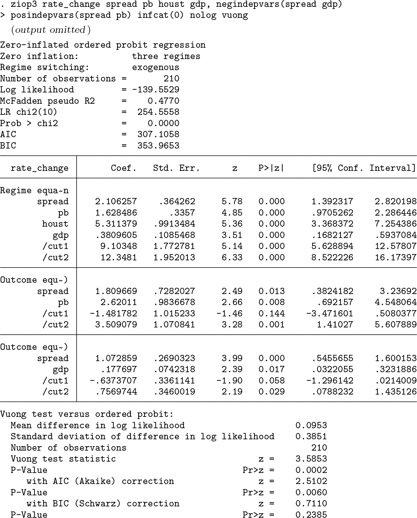
Next we allow for an inflation of zero outcomes and fit the three-part ZIOP-3 model. The ziop3 command with exogenous switching yields the following results:

The empirical evidence in favor of zero inflation is convincing: with only two extra parameters, the ZIOP-3 model has a much higher likelihood than the NOP model (−139.6 versus −151.0) and is clearly preferred by both AIC and BIC to the NOP and OP models. The Vuong tests for zero inflation (the standard one and one with the correction based on AIC) favor the ZIOP-3 model over the OP model at the 0.001 and 0.01 level, respectively. Endogenous switching does not significantly improve the likelihood of the ZIOP-3 model either (the p-value of the LR test of exogenous switching is 0.30, and both AIC and BIC prefer the exogenous switching).

In contrast, the likelihood of the two-part ZIOP-2 model is even lower than that of the NOP model. According to both AIC and BIC, the ZIOP-2 model is inferior to all the above models, including the OP one. The ziop2 command yields the following results:

The Vuong tests prefer the ZIOP-3 model to the ZIOP-2 model at the 0.01 significance level using the standard test statistic and at the 0.02 and 0.03 levels using the corrected statistics based, respectively, on AIC and BIC:

Now we report the selected output of the postestimation commands, performed for the ZIOP-3 model.

The predicted choice probabilities at the specified values of the independent variables can be estimated using the ziopprobabilities command:

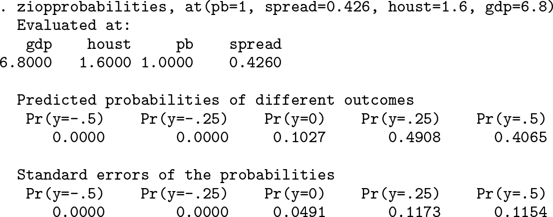
The predicted probabilities of the three latent regimes $s_{t}^{*} \in {- 1, 0, 1}$ or the probabilities of the three types of zeros conditional on each regime can be estimated for each sample observation by using the command predict with the option zeros or regimes, respectively:

The average predicted probabilities of the regimes s_t = −1, s_t = 0, and s_t = 1 in the sample are 0.40, 0.39, and 0.21, respectively. However, the average probability of zeros conditional on the regime s_t = −1 (0.15) is much higher than on the regime s_t = 1 (0.00).

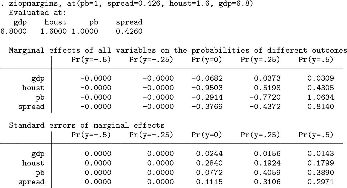
The marginal effects of the independent variables on the choice probabilities at the specified values of the independent variables can be estimated using the ziopmargins command:

The differences in the predicted choice probabilities (along with the standard errors) at two different values of the independent variables can be estimated using the ziopcontrasts command. In particular, this command may be used to compute the MEs of the discrete ordinal independent variables, such as pb (instead of using the ziopmargins command, which computes the derivatives of the probabilities):

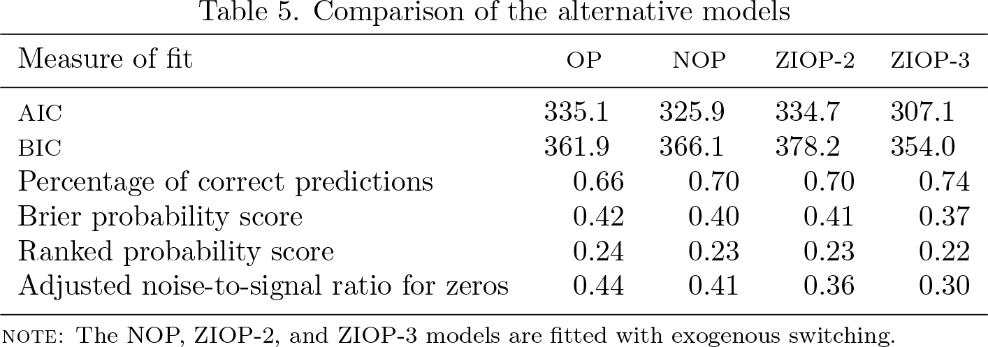
Finally, the different measures of model fit and the accuracy of the probabilistic predictions can be computed using the ziopclassification command:

As table 5 reports, the ZIOP-3 model demonstrates the best fit according to all the criteria.

Table 5.

Comparison of the alternative models

Measure of fit	OP	NOP	ZIOP-2	ZIOP-3
AIC	335.1	325.9	334.7	307.1
BIC	361.9	366.1	378.2	354.0
Percentage of correct predictions	0.66	0.70	0.70	0.74
Brier probability score	0.42	0.40	0.41	0.37
Ranked probability score	0.24	0.23	0.23	0.22
Adjusted noise-to-signal ratio for zeros	0.44	0.41	0.36	0.30

note: The NOP, ZIOP-2, and ZIOP-3 models are fitted with exogenous switching.

6 Concluding remarks

In this article, we described the ML estimation of the nested and cross-nested zero-inflated OP models using the new commands nop, ziop2, and ziop3. Such models can be applied to a variety of datasets in which the discrete ordinal outcomes can be divided into groups (nests) of similar choices, for example, the decisions to reduce, leave unchanged, or increase the choice variable (monetary policy interest rates, rankings, prices, consumption levels), or the negative, neutral, or positive attitudes to survey questions. The choice among the nests is driven by an ordered-choice switching mechanism that can be either exogenous or endogenous to the outcome decisions, which are also naturally ordered (large or small increase/decrease; disagree or strongly disagree; etc.). The models allow the probabilities of choices from different nests (for example, no change and an increase) to be driven by distinct mechanisms. Moreover, the cross-nested zero-inflated models allow the often abundant no-change or neutral outcomes to belong to all nests and be inflated by several different processes. The results of Monte Carlo simulations indicate that the proposed ML estimators are consistent and perform well in small samples.

Supplemental Material

Supplemental Material, sj-zip-1-stj-10.1177_1536867X211000002 - Estimation of nested and zero-inflated ordered probit models

Supplemental Material, sj-zip-1-stj-10.1177_1536867X211000002 for Estimation of nested and zero-inflated ordered probit models by David Dale and Andrei Sirchenko in The Stata Journal

Footnotes

7 Acknowledgments

We gratefully acknowledge support from the Basic Research Program of the National Research University Higher School of Economics in Moscow.

8 Programs and supplemental materials

To install a snapshot of the corresponding software files as they existed at the time of publication of this article, type

Notes

A Appendix

Table A1.

Monte Carlo experiments: The true values of parameters in the first set of simulations

	NOP (exog)	NOP	ZIOP-2 (exog)	ZIOP-2	ZIOP-3 (exog)	ZIOP-3
γ	(0.6, 0.4)^′	(0.6, 0.4)^′	(0.6, 0.8)^′	(0.6, 0.8)^′	(0.6, 0.4)^′	(0.6, 0.4)^′
µ	(0.21, 2.19)^′	(0.21, 2.19)^′	0.45	0.45	(0.9, 1.5)^′	(0.9, 1.5)^′
β			(0.5, 0.6)^′	(0.5, 0.6)^′
β⁻	(0.3, 0.9)^′	(0.3, 0.9)^′	(0.3, 0.9)^′	(0.3, 0.9)^′
β⁺	(0.2, 0.3)^′	(0.2, 0.3)^′	(0.2, 0.3)^′	(0.2, 0.3)^′
α			(−1.45, −0.55, 0.75, 1.65)^′	(−1.18, −0.33, 0.9, 1.76)^′
α⁻	−0.17	−0.5			(−0.67, 0.36)^′	(−0.88, 0.12)^′
α⁺	0.68	1.3			(0.02, 1.28)^′	(0.49, 1.67)^′
ρ			0	0.5
ρ⁻	0	0.3			0	0.3
ρ⁺	0	0.6			0	0.6

notes: (exog) means exogenous switching: ρ = ρ ⁻ = ρ ⁺ = 0. The variances σ 2 , σ − 2 , σ + 2 , and σ ν 2 are all fixed to 1 in all models.

References

Andrews

D. W. K.

2001. Testing when a parameter is on the boundary of the maintained hypothesis. Econometrica 69: 683–734. https://doi.org/10.1111/1468-0262.00210.

Andrews

D. W. K.

Cheng

2012. Estimation and inference with weak, semistrong, and strong identification. Econometrica 80: 2153–2211. https://doi.org/10.3982/ECTA9456.

Bagozzi

B. E.

Mukherjee

2012. A mixture model for middle category inflation in ordered survey responses. Political Analysis 20: 369–386. https://doi.org/10.1093/pan/mps020.

Basu

de Jong

2007. Dynamic multinomial ordered choice with an application to the estimation of monetary policy rules. Studies in Nonlinear Dynamics and Econometrics 11(4). https://doi.org/10.2202/1558-3708.1507.

Brier

G. W.

1950. Verification of forecasts expressed in terms of probability. Monthly Weather Review 78: 1–3. https://doi.org/10.1175/1520-0493(1950)078h0001:VOFEITi2.0.CO;2.

Brooks

Harris

M. N.

Spencer

2012. Inflated ordered outcomes. Economics Letters 117: 683–686. https://doi.org/10.1016/j.econlet.2012.08.020.

Clarke

K. A.

2003. Nonparametric model discrimination in international relations. Journal of Conflict Resolution 47: 72–93. https://doi.org/10.1177/0022002702239512.

Epstein

E. S.

1969. A scoring system for probability forecasts of ranked categories. Journal of Applied Meteorology and Climatology 8: 985–987. https://doi.org/10.1175/1520-0450(1969)008 h 0985:ASSFPF i 2.0.CO;2.

Famoye

Singh

K. P.

2003. On inflated generalized Poisson regression models. Advances and Applications in Statistics 3: 145–158.

10.

Greene

W. H.

1994. Accounting for excess zeros and sample selection in Poisson and negative binomial regression models. Working Paper 94-10, Stern School of Business, Department of Economics.

11.

Greene

W. H.

Hensher

D. A.

2010. Modeling Ordered Choices: A Primer. Cambridge: Cambridge University Press.

12.

Hall

D. B.

2000. Zero-inflated Poisson and binomial regression with random effects: A case study. Biometrics 56: 1030–1039. https://doi.org/10.1111/j.0006-341x.2000.01030.x.

13.

Hardin

J. W.

Hilbe

J. M.

2014. Estimation and testing of binomial and beta-binomial regression models with and without zero inflation. Stata Journal 14: 292–303. https://doi.org/10.1177/1536867X1401400204.

14.

Harris

M. N.

Zhao

2007. A zero-inflated ordered probit model, with an application to modelling tobacco consumption. Journal of Econometrics 141: 1073–1099. https://doi.org/10.1016/j.jeconom.2007.01.002.

15.

Heckman

J. J.

1978. Dummy endogenous variables in a simultaneous equation system. Econometrica 46: 931–959. https://doi.org/10.2307/1909757.

16.

Hernández

Drasgow

Gonzáles-Romá

2004. Investigating the functioning of a middle category by means of a mixed-measurement model. Journal of Applied Psychology 89: 687–699. https://doi.org/10.1037/0021-9010.89.4.687.

17.

Kaminsky

G. L.

Reinhart

C. M.

1999. The twin crises: The causes of banking and balance-of-payments problems. American Economic Review 89: 473–500. https://doi.org/10.1257/aer.89.3.473.

18.

Kelley

M. E.

Anderson

S. J.

2008. Zero inflation in ordinal data: Incorporating susceptibility to response through the use of a mixture model. Statistics in Medicine 27: 3674–3688. https://doi.org/10.1002/sim.3267.

19.

Kulas

J. T.

Stachowski

A. A.

2009. Middle category endorsement in odd-numbered Likert response scales: Associated item characteristics, cognitive demands, and preferred meanings. Journal of Research in Personality 43: 489–493. https://doi.org/10.1016/j.jrp.2008.12.005.

20.

Lambert

1992. Zero-inflated Poisson regression, with an application to defects in manufacturing. Technometrics 34: 1–14. https://doi.org/10.2307/1269547.

21.

Olsen

R. J.

1982. Distributional tests for selectivity bias and a more robust likelihood estimator. International Economic Review 23: 223–240. https://doi.org/10.2307/2526473.

22.

Silva

J. M. C. S.

2017. Local maxima in the estimation of the ZINB and sample selection models. UK Stata Users Group meeting proceedings. https://www.stata.com/meeting/uk17/slides/uk17_Santos_Silva.pdf.

23.

Sirchenko

2020. A model for ordinal responses with heterogeneous status quo outcomes. Studies in Nonlinear Dynamics and Econometrics 24(1). https://doi.org/10.1515/snde-2018-0059.

24.

Small

K. A.

1987. A discrete choice model for ordered alternatives. Econometrica 55: 409–424. https://doi.org/10.2307/1913243.

25.

Vovsha

1997. Application of cross-nested logit model to mode choice in Tel Aviv, Israel, metropolitan area. Transportation Research Record 1607: 6–15. https://doi.org/10.3141/1607-02.

26.

Vuong

Q. H.

1989. Likelihood ratio tests for model selection and non-nested hypotheses. Econometrica 57: 307–333. https://doi.org/10.2307/1912557.

27.

Wen

C.-H.

Koppelman

2001. The generalized nested logit model. Transportation Research, Part B 35: 627–641. https://doi.org/10.1016/S0191-2615(00)00045-X.

28.

Wilde

2000. Identification of multiple equation probit models with endogenous dummy regressors. Economics Letters 69: 309–312. https://doi.org/10.1016/S0165-1765(00)00320-7.

29.

Wilson

2015. The misuse of the Vuong test for non-nested models to test for zero-inflation. Economics Letters 127: 51–53. https://doi.org/10.1016/j.econlet.2014.12.029.

30.

Winkelmann

2008. Econometric Analysis of Count Data. 5th ed. Berlin: Springer.

Supplementary Material

Please find the following supplemental material available below.

For Open Access articles published under a Creative Commons License, all supplemental material carries the same license as the article it is associated with.

For non-Open Access articles published, all supplemental material carries a non-exclusive license, and permission requests for re-use of supplemental material or any part of supplemental material shall be sent directly to the copyright owner as specified in the copyright notice associated with the article.

0.00 MB