Fitting partially linear functional-coefficient panel-data models with Stata

Abstract

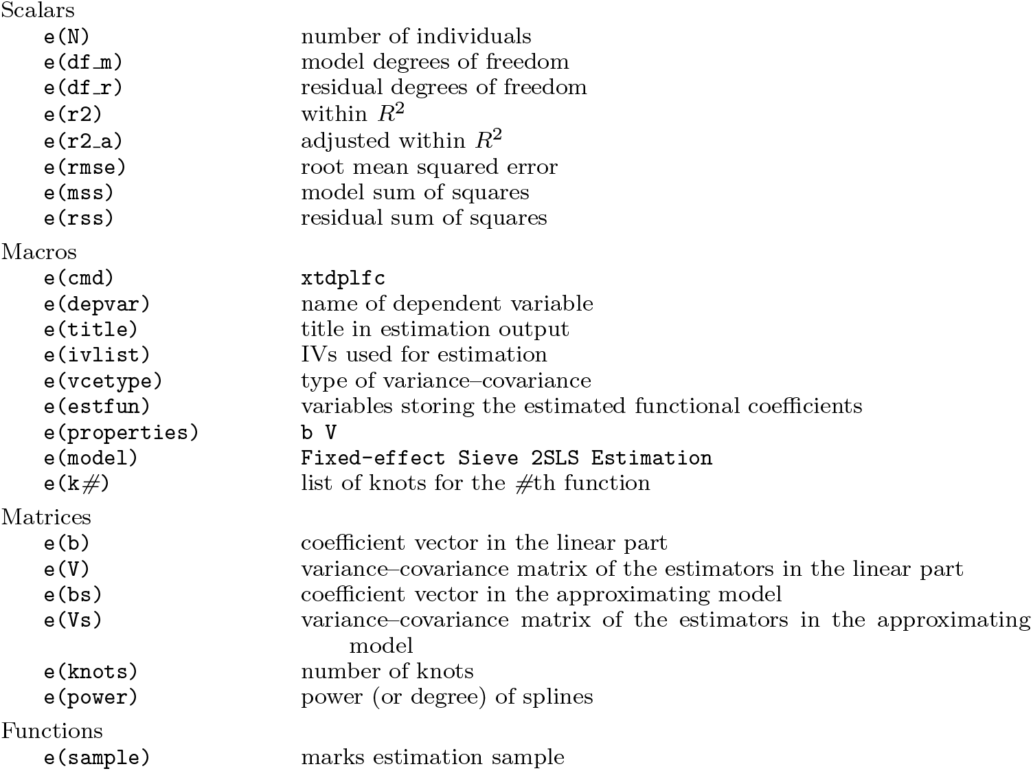
In this article, we describe the implementation of fitting partially linear functional-coefficient panel models with fixed effects proposed by An, Hsiao, and Li [2016, Semiparametric estimation of partially linear varying coefficient panel data models in Essays in Honor of Aman Ullah (Advances in Econometrics, Volume 36)] and Zhang and Zhou (Forthcoming, Econometric Reviews). Three new commands xtplfc, ivxtplfc, and xtdplfc are introduced and illustrated through Monte Carlo simulations to exemplify the effectiveness of these estimators.

1 Introduction

A partially linear functional-coefficient regression model allows for linearity in some regressors and nonlinearity in other regressors, where the effects of these covariates on the dependent variable vary according to a set of low-dimensional variables nonparametrically (Cai et al. 2017), thereby showing distinct advantages in capturing nonlinearity and heterogeneity. Through the seminal work of Chen and Tsay (1993), the functional-coefficient models have drawn much attention in the literature. To name a few, Cai, Fan, and Yao (2000), Cai, Fan, and Li (2000), and Cai, Li, and Park (2009) study functional-coefficient models under the time-series framework. Huang, Wu, and Zhou (2004) fit a functional-coefficient panel-data model without fixed effects via the series method. Cai and Li (2008) study functional-coefficient dynamic panel-data models without fixed effects based on the kernel method. Sun, Carroll, and Li (2009) consider functional-coefficient panel-data models with fixed effects that are removed via the least-square dummy variable approach. Alternatively, An, Hsiao, and Li (2016) deal with the fixed effects via the first time difference and fit the models using the series method. Zhang and Zhou (Forthcoming) propose to use a sieve two-step least square (2SLS) procedure to fit functional-coefficient panel dynamic models with fixed effects and develop a model specification test for the constancy of slopes.

In empirical studies, functional-coefficient models have been widely used. For example, they are applied to explore whether working experience matters to the impact of education on wage (Su, Murtazashvili, and Ullah 2013; Cai et al. 2017); to analyze the heterogeneous effect of foreign direct investment on economic growth (Delgado, Mc-Cloud, and Kumbhakar 2014; Cai et al. 2017); to examine the nonlinear relationship between income level and democracy (Lundberg, Huynh, and Jacho-Ch´avez 2017; Zhang and Zhou Forthcoming); to compare the returns to scale of the U.S. commercial banks across different regimes (Feng et al. 2017); and to investigate the role of marketization in China’s energy rebound effect (Li, Liu, and Du 2019).

The objective of this article is to present new commands to fit partially linear functional-coefficient panel-data models with fixed effects. The remainder of the article is organized as follows. Section 2 briefly describes the model and the estimation procedure. Sections 3–5 explain the syntax and options of the new commands. Section 6 provides some Monte Carlo simulations. Section 7 concludes the article.

2 The model

Consider a partially linear functional-coefficient panel-data model of the form

$Y_{it}=Z_{it}^{\prime }g\left(U_{it}\right)+X_{it}^{\prime }\beta +a_i+{\epsilon }_{it}i=1,\dots ,N,t=1,\dots ,T$

1

where the subscript i and t denote individual i and time t, respectively; Y_it is the scalar dependent variable; U _it = (U _{1 ,it},…, U_l,it )′ is a vector of continuous variables; Z _it = (Z _{1 ,it},…, Z_l,it )′ is a vector of covariates with functional coefficients g(U _it ) = {g ₁(U _{1 ,it} ),…, g_l (U_l,it )}′; X _it is a k × 1 vector of covariates with constant slopes β; and a_i is the individual fixed effects that might be correlated with Z _it , U _it , and X _it . ε_it represents the idiosyncratic error. Moreover, part of the elements in Z _it and X _it are allowed to be endogenous variables that are correlated with ε_it , and they could also include lagged dependent variables as in Zhang and Zhou (Forthcoming). ¹ In the latter case, (1) becomes a dynamic panel model with functional coefficients.

Recently, An, Hsiao, and Li (2016) and Zhang and Zhou (Forthcoming) propose using the series method to fit (1). The estimation procedure is sketched as follows.

First, one can use a linear combination of sieve basis functions to approximate the unknown functional coefficients in (1). Let h ^p (·) = {h_{p, 1}(·),…, h_{p,L p} (·)}′ be a L_p × 1 sequence of basis functions where the number of sieve basis functions L_p ≡ L_NL increases as either N or T increases. We have g_p (·) ≈ h ^p (·)′γ_p for p = 1,…, l, where γ_p = (γ_{p 1} ,…, γ_pLp ). Then, (1) can be rewritten as

$Y_{it}=H_{it}^{\prime }\Gamma +X_{it}^{\prime }\beta +a_i+v_{it}$

2

where H _it ≡ {Z _{1 ,it} h ¹(U _{1 ,it} )′,…, Z_l,it h ^l (U_l,it )′}′, Γ ≡ $\left({\gamma }_1^{\prime },\dots {\gamma }_l^{\prime }\right)\prime$ , and v_it = ε_it + r_it ,

$r_{it}=Z_{it}^{\prime }g\left(U_{it}\right)-H_{it}^{\prime }\Gamma$

denoting the sieve approximation error that becomes asymptotic negligible as L_p → ∞ for p = 1,…, l when (N, T) → ∞.

Then, taking the first time difference of (2) to eliminate the fixed effects yields

$\Delta Y_{it}=\Delta H_{it}^{\prime }\Gamma +\Delta X_{it}^{\prime }\beta +\Delta v_{it}$

3

where Δ represents a first-difference operator; that is, ΔA_t ≡ A_t − A_{t − 1}.

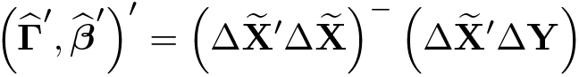
If all the variables are exogenous, (3) can be estimated through the least-squares method as in An, Hsiao, and Li (2016),

$\left(\widehat{\Gamma }\prime ,\widehat{\beta }\prime \right)\prime ={\left(\Delta \tilde{X}\prime \Delta \tilde{X}\right)}^{\_}\left(\Delta \tilde{X}\prime \Delta Y\right)$

where $\tilde{\mathbf{X}}$ = (X, H); X = $\left(X_1^{\prime },\dots ,X_N^{\prime }\right)\prime$ , X _i = (X_{i 1} ,…, X_iT )′; H = (H ₁ ,…, H _N )′, H _i = (H_{i 1} ,…, H_iT )′; and ⁻ denotes the generalized inverse.

If part of the variables in Z _it and X _it are endogenous, (3) can be estimated via the 2SLS method as in Zhang and Zhou (Forthcoming). Suppose we have a d × 1 vector of instrumental variables (ivs) with $d\ge \left({\displaystyle {\sum }_{p=1}^l{L}_p+k}\right)$ . The 2SLS estimator is given by

$\left(\widehat{\Gamma }.\widehat{\beta }\prime \right)\prime ={\left(\Delta \tilde{X}\prime P_W\Delta \tilde{X}\right)}^{-}\left(\Delta \tilde{X}\prime P_W\Delta Y\right)$

where P _W = W(W′W)⁻ W′ is a projection matrix with W being the IVs matrix.

Once $\tilde{\Gamma }$ is obtained, the functional coefficients g(U _it ) can be estimated by

${\widehat{g}}_P\left(U_{p,it}\right)=h^p\left(U_{p,it}\right)\prime \widehat{{\gamma }_P}p=1,\dots ,l$

Under certain regular assumptions, Zhang and Zhou (Forthcoming) establish the consistency and asymptotic normality of the above estimators when sample size N and T go to infinity jointly or only N tends to infinity.

In practice, there are several sieve methods to approximate the unknown functions. We follow Libois and Verardi (2013) to use the B-splines. More technical details on the B-splines can be found in Newson (2000b).

3 The xtplfc command

xtplfc fits An, Hsiao, and Li’s (2016) partially linear functional-coefficient panel-data models with exogenous variables.

3.1 Syntax

3.2 Options

zvars( varlist ) specifies variables that have functional coefficients. zvars() is required.

uvars( varlist ) specifies (continuous) variables that enter the functional coefficients interacted with variables in order specified by zvars(). uvars() is required.

generate( prefix ) specifies a prefix for the variable names to store fitted values of functional coefficients. generate() is required.

te specifies to include time fixed effects.

power( numlist ) (nonnegative integers) specifies the power (or degree) of the splines in order specified by uvars(). The default is power(3).

nknots( numlist ) specifies the number of knots used for the spline interpolation in order specified by uvars(). The default is nknots(2).

quantile specifies creating knots based on empirical quantiles. By default, the knots are generated by the rule of equal space.

maxnknots( numlist ) specifies the maximum number of knots used for conducting least-squares cross-validation (LSCV). If present, LSCV is used to determine the optimal number of knots. In our practice, we perform the leave-one-out cross-validation (CV) across the panelvar. That is to say, we leave one individual (with all observations during the sample period) out each time.

minnknots( numlist ) specifies the minimum number of knots used for performing LSCV. The default is minnknots(2).

grid( string ) specifies a prefix for the names to store the grid points of the variable specified by uvars( varlist ). If present, the functional coefficients are estimated over the grid points. By default, they are estimated over the observations.

pctile( # ) specifies the domain of the generating grid points. It can be used only when grid() is specified. The default is pctile(0).

brep( # ) specifies the number of bootstrap replications. The default is brep(200). We recommend that you select the number of replications.

wild specifies using the wild bootstrap. By default, residual bootstrap with the option cluster( panelvar ) is performed.

predict( prspec ) stores predicted values of the conditional mean and fixed effects using variable names specified in prspec. Specifically, one uses predict( varlist | stub * [, replace noai]). The option takes a variable list or stub. The first variable name corresponds to the predicted conditional mean. The second name corresponds to fixed effects. When replace is used, variables with the names in varlist or stub * are replaced by those in the new computation. If noai is specified, only a variable for the mean is created.

nodots suppresses the iteration dots.

level( # ) sets the confidence level. The default is level(95).

fast speeds up using Mata functions.

tenfoldcv specifies using tenfold CV instead of LSCV. It is done by dividing the sample into 10 pieces and conducting LSCV across these 10 pieces. Specifically, given the number of knots, leave one piece out, run the regression using the left pieces, and predict the dependent variable for the remaining piece.

3.3 Stored results

xtplfc stores the following in e():

3.4 Dependency of xtplfc

xtplfc depends on the moremata (Jann 2005) and bspline (Newson 2000a) packages.

4 The ivxtplfc command

ivxtplfc fits Zhang and Zhou’s (Forthcoming) partially linear functional-coefficient panel-data models with endogenous variables using the sieve 2SLS method.

4.1 Syntax

4.2 Options

zvars( varlist ) specifies variables that have functional coefficients. zvars() is required.

uvars( varlist ) specifies (continuous) variables that enter the functional coefficients interacted with variables in order specified by zvars(). uvars() is required.

generate( prefix ) specifies a prefix for the names to store fitted values of functional coefficients. generate() is required.

endox( varlist ) specifies endogenous variables that enter the model linearly.

endozflag( numlist ) specifies the orders of variables in zvars( varlist ) that are endogenous variables. For example, endozflag(1 3) indicates that the first and third variables specified in zvars( varlist ) are endogenous.

ivx( varlist ) specifies IVs that enter the model linearly.

ivz( varlist , uflag( numlist ) [ivtype( numlist )]) specify IVs entering the model nonlinearly that interact with the functions specified by the orders in uflag( numlist ). Optionally, one may specify the type of nonlinear IVs to be constructed. iv-type( numlist ) means using the #th lag of the basis functions, and the final IVs are formed from ivz()× L#.S(u) [where S(u) are basis functions of u]. By default, the first lag of the basis functions is used.

te specifies to include time fixed effects.

power( numlist ) (nonnegative integers) specifies the power (or degree) of the splines in order specified by uvars(). The default is power(3).

nknots( numlist ) specifies the number of knots used for the spline interpolation in order specified by uvars(). The default is nknots(2).

quantile specifies creating knots based on empirical quantiles. By default, the knots are generated by the rule of equal space.

maxnknots( numlist ) specifies the maximum number of knots used for conducting LSCV. If present, LSCV is used to determine the optimal number of knots. In our practice, we perform the leave-one-out CV across the panelvar. That is to say, we leave one individual (with all observations during the sample period) out each time.

minnknots( numlist ) specifies the minimum number of knots used for performing LSCV. The default is minnknots(2).

grid( string ) specifies a prefix for the names to store the grid points of the variable specified by uvars(). If present, the functional coefficients are estimated over the grid points. By default, they are estimated over the observations.

pctile( # ) specifies the domain of the generating grid points. It can be used only when grid() is specified. The default is pctile(0).

brep( # ) specifies the number of bootstrap replications. The default is brep(200). We recommend that you select the number of replications.

wild specifies using the wild bootstrap. By default, residual bootstrap with the option cluster( panelvar ) is performed.

predict( prspec ) stores predicted values of the conditional mean and fixed effects using variable names specified in prspec. Specifically, one uses predict( varlist | stub * [, replace noai]). The option takes a variable list or stub. The first variable name corresponds to the predicted conditional mean. The second name corresponds to fixed effects. When replace is used, variables with the names in varlist or stub * are replaced by those in the new computation. If noai is specified, only a variable for the mean is created.

nodots suppresses the iteration dots.

level( # ) sets the confidence level. The default is level(95).

fast speeds up using Mata functions.

tenfoldcv specifies using tenfold CV instead of LSCV.

4.3 Stored results

ivxtplfc stores the following in e():

4.4 Dependency of ivxtplfc

ivxtplfc depends on the moremata (Jann 2005) and bspline (Newson 2000a) packages.

5 The xtdplfc command

xtdplfc fits Zhang and Zhou’s (Forthcoming) partially linear functional-coefficient panel dynamic data models using the sieve 2SLS method.

5.1 Syntax

5.2 Options

uvars( varlist ) specifies (continuous) variables that enter the functional coefficients interacted with variables in order specified by zvars(). uvars() is required.

generate( prefix ) specifies a prefix for the names to store fitted values of functional coefficients. generate() is required.

zvars( varlist ) specifies variables that have functional coefficients.

lags( # ) specifies using # lags of the dependent variable as covariates. The default is lags(1).

lagyinz( numlist ) specifies lags of the dependent variable that have functional coefficients. When this option is used, the specified lags of the dependent variable are automatically added in front of variables in zvars().

endox( varlist ) specifies endogenous variables that enter the model linearly.

endozflag( numlist ) specifies the orders of variables in zvars( varlist ) that are endogenous variables. For example, endozflag(1 3) indicates that the first and third variables specified in zvars( varlist ) are endogenous.

ivx( varlist ) specifies IVs that enter the model linearly.

ivz( varlist , uflag( numlist ) [ivtype( numlist )]) specify IVs entering the model non-linearly that interact with the functions specified by the orders in uflag( numlist ). Optionally, one may specify the type of nonlinear IVs to be constructed. iv-type( numlist ) means using the #th lag of the basis functions, and the final IVs are formed from ivz()× L#.S(u) [where S(u) are basis functions of u]. By default, the first lag of the basis functions is used.

onlyivxz uses only instruments specified by ivx() and ivz(). By default, additional instruments are automatically constructed using lags of the dependent variables, variables specified by endox() and endozflag(), and the generating splines.

ivtype( numlist ) specifies the lag of the basis functions to be used for constructing the IVs. Suppose Z is an endogenous variable interacting with g(U); S(U) are basis functions for g(U). ivtype(1) indicates constructing IVs from L2.Z × L.S(U).

te specifies to include time fixed effects.

power( numlist ) (nonnegative integers) specifies the power (or degree) of the splines in order specified by uvars(). The default is power(3).

nknots( numlist ) specifies the number of knots used for the spline interpolation in order specified by uvars(). The default is nknots(2).

quantile specifies creating knots based on empirical quantiles. By default, the knots are generated by the rule of equal space.

maxnknots( numlist ) specifies the maximum number of knots used for conducting LSCV. If present, LSCV is used to determine the optimal number of knots. In our practice, we perform the leave-one-out CV across the panelvar. That is to say, we leave one individual (with all observations during the sample period) out each time.

minnknots( numlist ) specifies the minimum number of knots used for performing LSCV. The default is minnknots(2).

grid( string ) specifies the name for storing the grid points of the variable specified by uvars(). If present, the functional coefficients are estimated over the grid points. By default, they are estimated over the observations.

pctile( # ) specifies the domain of the generating grid points. It can be used only when grid() is specified. The default is pctile(0).

brep( # ) specifies the number of bootstrap replications. The default is brep(200). We recommend that you select the number of replications.

wild specifies using the wild bootstrap. By default, residual bootstrap with the option cluster( panelvar ) is performed.

predict( prspec ) stores predicted values of the conditional mean and fixed effects using variable names specified in prspec. Specifically, one uses predict( varlist | stub * [, replace noai]). The option takes a variable list or stub. The first variable name corresponds to the predicted conditional mean. The second name corresponds to fixed effects. When replace is used, variables with the names in varlist or stub * are replaced by those in the new computation. If noai is specified, only a variable for the mean is created.

nodots suppresses the iteration dots.

level( # ) sets the confidence level. The default is level(95). fast speeds up using Mata functions.

tenfoldcv specifies using tenfold CV instead of LSCV.

5.3 Stored results

xtdplfc stores the following in e():

5.4 Dependency of xtdplfc

xtdplfc depends on the moremata (Jann 2005) and bspline (Newson 2000a) packages.

6 Monte Carlo simulation

In this section, we investigate the finite sample performance of estimators discussed above through Monte Carlo simulations. For all data-generating processes (DGPs) to be considered, we set up a standard fixed-effects panel comprising 50 individuals over 40 time periods; that is, N = 50, T = 40. We carry out 500 replications.

We first consider the static panel-data model as follows (DGP1):

$Y_{it}{=X}_{1,it}{-X}_{2,it}{+g(X}_{3,it}{)Z}_{it}{+a}_{\text{i}}{+\epsilon }_{it}{g(X}_{3,it}{)=X}_{3,it}{+2(X}_{3,it}{\text{)}}^2-0{\text{.25}(X}_{3,it}{\text{)}}^{\text{3}}$

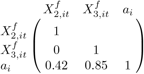
Following Libois and Verardi (2013), we generate X _{1 ,it} , X _{2 ,it} , X _{3 ,it} , and a_i via a two-step procedure ² as follows:

$\begin{array}{l}{X}_{1,it}=X_{1,it}^e\\ X_{2,it}=\left(X_{2,i}^f+X_{2,it}^e\right)/\sqrt{2}\\ X_{3,it}=\left(X_{3,i}^f+X_{3,it}^e\right)/\sqrt{2}\end{array}$

We draw $X_{2,it}^f,X_{3,it}^f$ , and a_i from the multivariate normal distribution with mean µ = (0, 0, 0) and covariance matrix

$\begin{array}{ll}\begin{array}{l} \\ X_{2,it}^f\\ X_{3,it}^f\\ a_i\end{array}\hfill & \begin{array}{c}\begin{array}{lll}{X}_{2,it}^f\hfill & X_{3,it}^f\hfill & a_i\hfill \end{array}\\ \left(\begin{array}{lll}\begin{array}{l}1\\ 0\\ 0,42\end{array}\hfill & \begin{array}{l} \\ 1\\ 0.85\end{array}\hfill & \begin{array}{l} \\ \\ 1\end{array}\hfill \end{array}\right)\end{array}\hfill \end{array}$

Similarly, $X_{1,it}^e,X_{2,it}^e$ , and $X_{3,it}^e$ are drawn from the multivariate normal distribution with mean µ = (0, 0, 0) and covariance matrix

$\begin{array}{ll}\begin{array}{l} \\ X_{1,it}^e\\ X_{2,it}^e\\ X_{3,it}^e\end{array}\hfill & \begin{array}{c}\begin{array}{lll}{X}_{1,it}^e\hfill & X_{2,it}^e\hfill & X_{3,it}^e\hfill \end{array}\\ \left(\begin{array}{lll}\begin{array}{l}1\\ 0.2\\ 0,8\end{array}\hfill & \begin{array}{l} \\ 1\\ 0\end{array}\hfill & \begin{array}{l} \\ \\ 1\end{array}\hfill \end{array}\right)\end{array}\hfill \end{array}$

For comparison, we consider the following three regression models.

Model 1: xtplfc, considering that X _{1 ,it} and X _{2 ,it} enter the model linearly, whereas Z_it is included with a functional coefficient of X _{3 ,it} .

Model 2: xtreg, regressing Y_it on X _{1 ,it} , X _{2 ,it} , X _{3 ,it} , and Z_it with fixed effects.

Model 3: xtreg, regressing Y_it on X _{1 ,it} , X _{2 ,it} , X _{3 ,it} , Z_it , and c.X _{3 ,it} #c.Z_it with fixed effects.

The simulation codes for DGP 1 are presented as follows: ³

Following Burton et al. (2006) and White (2010), we report the bias, mean square error (MSE), median width of 95% confidence interval, and coverage of 95% confidence interval of the estimated coefficients associated with X _{1 ,it} and X _{2 ,it} in table 1. We find that the fixed-effects sieve estimator outperforms the fixed-effects estimator in terms of both bias and MSE. As expected, the bias is relatively large in models 2 and 3 because they suffer from endogeneity due to omitting the nonlinear relationship of X _{3 ,it} and Z_it . In terms of the 95% confidence interval, the fixed-effects sieve estimator gives rise to a relatively small interval width. Moreover, coverage probabilities of 95% confidence interval generated by the fixed-effects sieve estimator are quite close to the nominal value (0.95). The average fit of g(X_it ) with the corresponding 95% confidence band in the simulations is presented in figure 1. We see that the average fit is very close to the true function g(X_it ) and that the 95% confidence band is relatively small except for the edges.

Table 1.

Simulation results for the parametric parts in DGP 1

	Bias		MSE		95% CI width		Coverage
	X1 ,it	X2 ,it	X1 ,it	X2 ,it	X1 ,it	X2 ,it	X1 ,it	X2 ,it
Model 1	0.0016	0.0026	0.0007	0.0014	0.1084	0.1559	0.9540	0.9560
Model 2	−0.0547	−0.0769	0.0045	0.0071	0.5667	0.4891	1.0000	1.0000
Model 3	−0.0830	-0.0605	0.0084	0.0048	0.5595	0.4828	1.0000	1.0000

Figure 1.

Average fit of g(X ₃) across replications

Next, we consider the case of dynamic panel data (DGP2):

$\begin{array}{c}{Y}_{it}=g\left(U_{it}\right)Y_{it-1}+0,3Y_{it-2}+0.3X_{it}+a_i+{\epsilon }_{it}\\ g\left(U_{it}\right)=\sin \left(\frac{\pi }{3}{U}_{it}\right)\\ X_{it}=W_{it}+0.5a_i\end{array}$

We assume ε_it are independent and identically distributed (IID) N(0, 1) across both i and t and a_i are IID N(0, 1). W_it and U_it are drawn from IID U(0, 10) and IID U(−9, 9), respectively.

We compare the performance of ivxtplfc and ivregress 2sls via the following models:

Model 4: ivxtplfc, considering that X_it and Y_{it − 2} enter the model linearly, whereas Y_{it − 1} is included with a functional coefficient of U_it .

Model 5: ivregress 2sls, taking first difference to remove fixed effects and regressing ΔY_it on ΔY_{it − 1}, ΔY_{it − 2}, and ΔX_it .

Model 6: ivregress 2sls, taking first difference to remove fixed effects and regressing ΔY_it on ΔY_{it − 1}, ΔY_{it − 2}, ΔX_it , and ΔU_it .

Note that L2.Y_it (the second lag of Y_it ) is used as the IV in ivregress 2sls and that the interaction of L2.Y_it and the first lag of the basis functions of U_it is constructed as the IVs in ivxtplfc. The simulation codes for DGP 2 are presented as follows:

Table 2 presents the bias, mean square error (MSE), median width of 95% confidence interval, and coverage of 95% confidence interval of the estimated coefficients associated with Y_{it − 2} and X_it . Similar to DGP1, the simulation results show that the fixed-effects sieve 2SLS estimator performs much better than the fixed-effects 2SLS estimator in terms of bias, MSE, width of 95% confidence interval, and coverage of 95% confidence interval. Figure 2 displays the average fit of g(U_it ) with the corresponding 95% band in the simulations. Although g(U_it ) is fluctuated greatly in model 4, the proposed method estimates it quite well.

Table 2.

Simulation results for the parametric parts in DGP 2

	Bias		MSE		95% CI width		Coverage
	Yit − 2	Xit	Yit − 2	Xit	Yit − 2	Xit	Yit − 2	Xit
Model 4	−0.0009	−0.0005	0.0002	0.0002	0.0542	0.0527	0.9360	0.9400
Model 5	0.0302	0.0357	0.0017	0.0018	0.3623	0.2555	1.0000	1.0000
Model 6	0.0266	0.0385	0.0015	0.0020	0.3603	0.2539	1.0000	1.0000

Figure 2.

Average fit of g(U) across replications

7 Conclusion

Popular in academic research, partially linear functional-coefficient models are flexible enough to accommodate the nonlinear structure and capture the heterogeneity over individuals and times. This article briefly introduced the new development of functional-coefficient panel-data models and provided three new commands for implementing estimation. Additionally, we illustrated the usefulness of our proposed commands via some simple simulations.

Supplemental Material

Supplemental Material, st0624 - Fitting partially linear functional-coefficient panel-data models with Stata

Supplemental Material, st0624 for Fitting partially linear functional-coefficient panel-data models with Stata by Kerui Du, Yonghui Zhang and Qiankun Zhou in The Stata Journal

References

1.
AnY.HsiaoC.LiD.. 2016. Semiparametric estimation of partially linear varying coefficient panel data models. In Essays in Honor of Aman Ullah (Advances in Econometrics, Volume 36), ed. Gonz´alez-RiveraG.HillR. C.LeeT.-H., 47–65. Bingley, UK: Emerald. https://doi.org/10.1108/S0731-905320160000036011.
2.
BaumC. F.AzevedoJ. P.. 2001. outtable: Stata module to write matrix to LATEX table. Statistical Software Components S419501, Department of Economics, Boston College. https://ideas.repec.org/c/boc/bocode/s419501.html.
3.
BurtonA.AltmanD. G.RoystonP.HolderR. L.. 2006. The design of simulation studies in medical statistics. Statistics in Medicine25: 4279–4292. https://doi.org/10.1002/sim.2673.
4.
CaiZ.FanJ.LiR.. 2000. Efficient estimation and inferences for varying-coefficient models. Journal of the American Statistical Association95: 888–902. https://doi.org/10.1080/01621459.2000.10474280.
5.
CaiZ.FanJ.YaoQ.. 2000. Functional-coefficient regression models for nonlinear time series. Journal of the American Statistical Association95: 941–956. https://doi.org/10.1080/01621459.2000.10474284.
6.
CaiZ.FangY.LinM.SuJ.. 2017. Inferences for a partially varying coefficient model with endogenous regressors. Journal of Business & Economic Statistics37: u. https://doi.org/10.1080/07350015.2017.1294079.
7.
CaiZ.LiQ.. 2008. Nonparametric estimation of varying coefficient dynamic panel data models. Econometric Theory24: 1321–1342. https://doi.org/10.1017/S0266466608080523.
DelgadoM. S.McCloudN.KumbhakarS. C.. 2014. A generalized empirical model of corruption, foreign direct investment, and growth. Journal of Macroeconomics42: 298–316. https://doi.org/10.1016/j.jmacro.2014.09.007.
11.
FengG.GaoJ.PengB.ZhangX.. 2017. A varying-coefficient panel data model with fixed effects: Theory and an application to US commercial banks. Journal of Econometrics196: 68–82. https://doi.org/10.1016/j.jeconom.2016.09.011.
12.
HuangJ. Z.WuC. O.ZhouL.. 2004. Polynomial spline estimation and inference for varying coefficient models with longitudinal data. Statistica Sinica14: 763–788.
13.
JannB.2005. moremata: Stata module (Mata) to provide various functions. Statistical Software Components S455001, Department of Economics, Boston College. https://ideas.repec.org/c/boc/bocode/s455001.html.
14.
LiJ.LiuH.DuK.. 2019. Does market-oriented reform increase energy rebound effect? Evidence from China’s regional development. China Economic Review56: 101304. https://doi.org/10.1016/j.chieco.2019.101304.
LundbergA. L.HuynhK. P.Jacho-Ch´avezD. T.. 2017. Income and democracy: A smooth varying coefficient redux. Journal of Applied Econometrics32: 719–724. https://doi.org/10.1002/jae.2536.
17.
NewsonR. B.2000a. bspline: Stata modules to compute B-splines parameterized by their values at reference points. Statistical Software Components S411701, Department of Economics, Boston College. https://ideas.repec.org/c/boc/bocode/s411701.html.
18.
NewsonR. B.2000b. sg151: B-splines and splines parameterized by their values at reference points on the x-axis. Stata Technical Bulletin57: 20–27. Reprinted in Stata Technical Bulletin Reprints. Vol. 10, pp. 221–230. College Station, TX: Stata Press.
SuL.MurtazashviliI.UllahA.. 2013. Local linear GMM estimation of functional coefficient IV models with an application to estimating the rate of return to schooling. Journal of Business & Economic Statistics31: 184–207. https://doi.org/10.1080/07350015.2012.754314.
21.
SunY.CarrollR. J.LiD.. 2009. Semiparametric estimation of fixed-effects panel data varying coefficient models. In Nonparametric Econometric Methods, ed. LiQ.RacineJ. S., 101–129. Bingley, UK: Emerald. https://doi.org/10.1108/S0731-9053(2009)0000025022.
ZhangY.ZhouQ.. Forthcoming. Partially linear functional-coefficient dynamic panel data models: Sieve estimation and specification testing. Econometric Reviews.
Supplementary Material
Please find the following supplemental material available below.
For Open Access articles published under a Creative Commons License, all supplemental material carries the same license as the article it is associated with.
For non-Open Access articles published, all supplemental material carries a non-exclusive license, and permission requests for re-use of supplemental material or any part of supplemental material shall be sent directly to the copyright owner as specified in the copyright notice associated with the article.