Using information from singletons in fixed-effects estimation: xtfesing

Abstract

In this article, we describe the xtfesing command. The command implements a generalized method of moments estimator that allows exploiting singleton information in fixed-effects panel-data regression as in Bruno, Magazzini, and Stampini (2020, Economics Letters 186: Article 108519).

1 Introduction

Analysis of longitudinal (panel) data has the advantage of allowing consistent estimation of the model parameters even in the presence of unobserved heterogeneity, that is, of decreasing the risk of omitted variables bias. The fixed-effects approach (in Stata, the xtreg command with the fe option) allows estimating the effect of time-varying variables even in the presence of correlation with the error term, provided that the correlation is driven by omitted time-invariant variables, either observed or unobservable (such as individual preferences or gender or firms’ propensity to patent or foundation year). Consistent estimation of the parameters of interest is obtained by using the within-group transformation that removes the individual average from the variables included in the model. Singleton units, that is, those units observed only at one point in time, do not contribute to the analysis, because their within-group transformation is identically equal to zero.

While most textbook examples consider a balanced panel dataset, real data often entail an unbalanced set of units, with a substantial share of singleton observations. In some cases, singletons are due to natural enterprise mortality and refreshment of the sample with new units. This type of attrition is common in databases like Orbis (https://www.bvdinfo.com/en-gb) or the Business Environment and Enterprise Performance Survey (https://www.beeps-ebrd.com/data; https://www.enterprisesurveys.org/). In the case of rotating panels, singletons are the result of the sampling framework. This happens in many labor force surveys in which a share of the observations is replaced in each wave, and the observations that are interviewed only in the first wave are singletons by design. Attrition and singletons can also be due to the death of part of the sample. This is particularly relevant for samples of older people, as in the United States’ Health and Retirement Study (https://hrs.isr.umich.edu/about) or the Mexican Health and Aging Study (http://www.mhasweb.org/). Migration and nonresponse are other common causes of attrition and the resulting presence of singleton observations in longitudinal data.

In this article, we describe the xtfesing command, which estimates a static panel-data model with fixed effects and exploits information from the singleton units in the sample with the aim to increase estimation efficiency. The methodology has been proposed by Bruno, Magazzini, and Stampini (2020). The method can also be used to “pool” panel datasets and cross-section observations from other survey waves as in Bruno and Stampini (2009).

xtfesing implements a two-step generalized method of moments (GMM) estimator (Hansen 1982). Its validity relies on the homogeneity assumption: it requires that the ordinary least-squares (OLS) bias be the same for the panel units and the singletons.

The article proceeds as follow. Section 2 describes the methodology. Section 3 presents the syntax of the xtfesing command, its estimation options, and its postestimation characteristics. Section 4 provides an example based on the Stata dataset nlswork.dta.

2 Method

Consider the linear static panel-data model with individual effects (i = 1,…, N; t = 1,…, T_i ),

$y_{it}={{\text{x}}^{\prime }}_{it}\beta +u_i+e_{it}$

1

where y_it represents the dependent variable of interest measured on unit i at time t, x _it a k × 1 vector of observable characteristics of unit i at time t (an intercept can be included), β a k × 1 vector of parameters to be estimated, u_i the individual effect, and e_it the idiosyncratic component. The variables in x _it are allowed to be arbitrarily correlated with u_i , but the assumption of strict exogeneity is imposed so that correlation of x _it with e_is is ruled out at any time (s = 1,…, T_i ). The panel can be unbalanced: the number of time-period observations for unit i equals T_i .

In the setup of (1), the fixed-effects estimator is consistent: the presence of an unbalanced¹ panel complicates only the notation but does not affect the properties of the estimator.

Define ${\ddot{x}}_{j,it}=x_{j,it}-{\overline{x}}_{j,i}$ with ${\overline{x}}_{j,i}={\sum }_t{x}_{j,it}/T_i\left(j=1,\mathrm{....},k\right),$ the individual demeaned independent variables. In the case of T_i = 1 (singleton units), ẍ _j,it = 0 for each regressor j. The fixed-effects estimator can be obtained as an instrumental variable estimator of (1) with instruments ẍ _j,it . The following k moment conditions are therefore satisfied [see (2) in Bruno, Magazzini, and Stampini (2020)]: ²

$E\left\{{\ddot{x}}_{j,it}\left(y_{it}-{\text{x}}_{it}^{\prime }\beta \right)\right\}=0$

2

In contrast, because of the possibility of correlation between the independent variables and the individual component u_i , the OLS estimator may be biased. Denote with b the OLS bias; also, the following moment conditions are satisfied [see (2) in Bruno, Magazzini, and Stampini (2020)]:

$E\left[x_{it}\left\{y_{it}-{\text{x}}_{it}^{\prime }\left(\beta +b\right)\right\}\right]=0$

3

As an equal number of moment conditions and parameters are added, the estimated coefficients in β are unaffected. However, information from singleton units can be further exploited to obtain efficiency gains under the assumption that the OLS bias is the same for the singletons and those units that are observed more than once. Denote with i = s the singletons: the following moment condition can also be considered [see (3) in Bruno, Magazzini, and Stampini (2020)]:

$E\left[{\text{x}}_{st}\left\{y_{st}-{\text{x}}_{st}^{\prime }\left(\beta +b\right)\right\}\right]=0$

4

We propose a GMM estimator based on moment conditions (2), (2), and (3). The computation considers a two-step procedure based on the gmm Stata command with clustered standard errors (cluster defined on the basis of the group variable that identifies the units). It includes Windmeijer’s (2005) formula for the correction of the two-step estimated standard error.

The assumption of homogeneity can be tested using a regression framework or on the basis of the test of overidentifying conditions based on the value of the minimized GMM criterion. The two test statistics are provided with the proposed command. Please refer to Bruno, Magazzini, and Stampini (2020) for details.

3 The xtfesing command

3.1 Syntax

The syntax of the xtfesing command is as follows:

depvar represents the dependent variable, and indepvars the list of independent variables. A subsample of the data can be specified using the if or in qualifier, as usual.

3.2 Options

id(varname) specifies varname identifying the grouping variable. The option can be omitted when the variables identifying the panel dimensions have been specified with the xtset command. In this case, the variable identifying the panel units is considered (if the option is omitted but no xtset command has been defined before xtfesing, an error message is displayed).

nowindmeijer specifies that the default standard errors computed by Stata’s gmm command be reported. By default, they are computed using Windmeijer’s (2005) correction.

level(#) specifies the confidence level. The default is level(95).

3.3 Postestimation command

The xtfesing command allows the use of the postestimation command predict. The following options can be specified:

xb a + x^′ β, fitted values (the default)

ue u_i + e_it , the combined residual

3.4 Stored results

xtfesing stores the following results in e():

4 Example: A wage equation

We consider nlswork.dta, available online from the Stata website: ³

. webuse nlswork

(National Longitudinal Survey. Young Women 14-26 years of age in 1968)

The dataset contains information on young women between the ages of 14 and 26 in 1968. Data are extracted from the National Longitudinal Surveys conducted by the U.S. Department of Labor.

We specify the panel dimensions by using the xtset command:

The dataset contains 4,711 units observed over 15 time periods (from 1968 to 1988, with some gaps). The panel is unbalanced: a description of the dataset structure with xtdescribe yields the following results:

The two most common patterns are indeed singletons: 136 units are observed only in the first time period, and 114 are observed only in the last time period. Singletons also include units with a single observation at any intermediate time, plus units with more than one observation that enter the estimation sample only once because of missing values in the variables considered by the model. This last group is not counted with xtdescribe, which is based on the number of lines occupied by each unit in the dataset.

We consider the logarithm of wage (ln_wage) as dependent variable and include among the independent variables total work experience (ttl_exp) and its square, a dummy variable for union membership (union), the age of the woman, and three dummy variables to identify her residence (south, c_city, and not_smsa).

We first generate the square of the variable ttl_exp:

. generate ttl_exp2 = ttl_exp^2

As a benchmark for the proposed estimation procedure, we also consider the fixed- effects estimator. Robust standard error, clustered over idcode, is considered to account for the possibility of heteroskedasticity and autocorrelation in the idiosyncratic component. Some missing values are present, so the number of units decreases to 4,150. ⁴

Overall, the estimation sample includes 665 singletons: the presence of singletons is reflected in the number of years of observations, which ranges from 1 to 12.

The same equation is estimated using the Bruno, Magazzini, and Stampini (2020) procedure implemented with the xtfesing command:

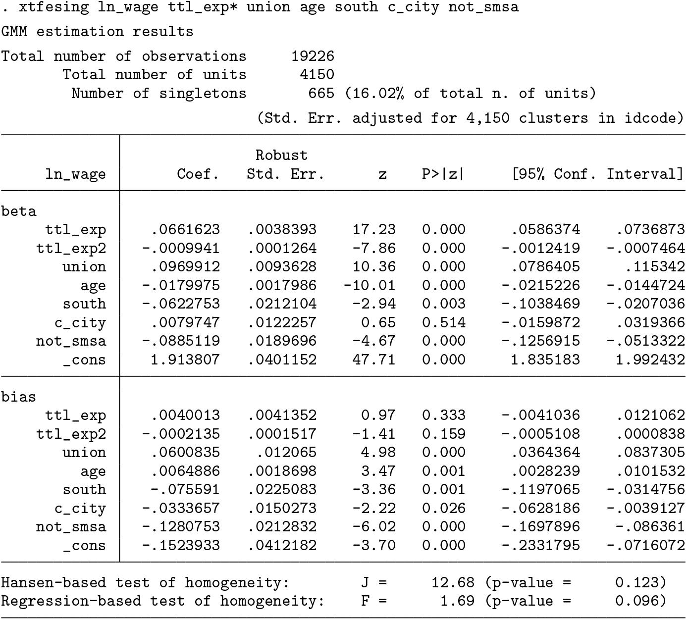
The option id() is omitted because we previously defined the panel through the command xtset. The variable idcode is therefore considered to identify the units.

At the top of the table of results, we have information on the total number of observations (19,226), the total number of units (4,150) and the number of singletons (665, corresponding to 16.02% of the total number of units).

The table of results reports the estimated coefficients for “beta” (the consistent estimator of the coefficient of interest) and the OLS “bias” for each variable in the estimated equation. Note that when the predict command is invoked after xtfesing, only the coefficients in “beta” are considered for computing predicted values and residuals (coefficients in “bias” are not included in the computations).

At the bottom, the table reports the two tests of the homogeneity assumption, required for the validity of the proposed approach:

The Hansen-based test of homogeneity, corresponding to the test of overidentifying restrictions for the GMM estimation, produces a value of 12.68 with a p-value of 0.123.

The regression-based test of homogeneity produces a value of 1.69 with a p-value of 0.096.

Both tests do not reject the null hypothesis of homogeneity at the 5% level of significance, so the Bruno, Magazzini, and Stampini (2020) procedure can be applied to these data.

In this case, the reduction in the standard errors is limited (or null). As Bruno, Magazzini, and Stampini (2020) point out, efficiency gains can be negligible with a long time dimension or when the share of singletons is not substantial.

For illustration, we limit the analysis to the last three years of the dataset (85, 87, and 88). We also restrict the sample by only including white women. In this way, we “artificially” generate a dataset characterized by a small time dimension and a larger (even though, still fairly limited) share of singletons.

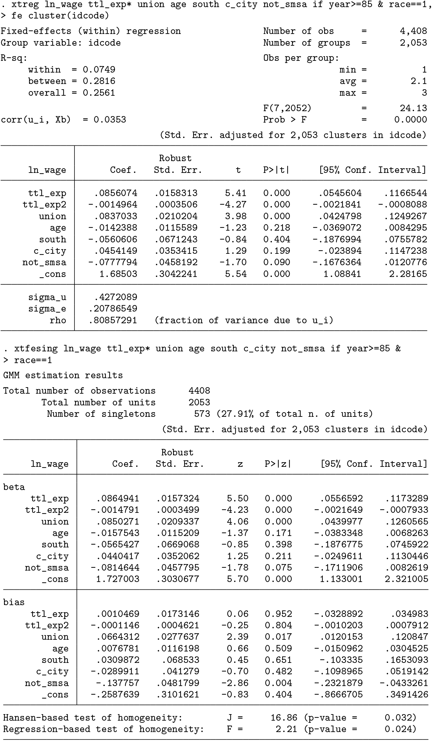
In this case, standard errors tend to be lower when using xtfesing as compared with xtreg. The homogeneity assumption is not rejected at the 1% level of significance.

Bruno, Magazzini, and Stampini (2020) consider cases in which the share of singletons reaches or exceeds 50%. They show that, in those cases, the procedure implemented by xtfesing leads to large improvements in estimation efficiency.

Supplemental Material

Supplemental Material, st0623 - Using information from singletons in fixed-effects estimation: xtfesing

Supplemental Material, st0623 for Using information from singletons in fixed-effects estimation: xtfesing by Laura Magazzini, Randolph Luca Bruno and Marco Stampini in The Stata Journal