Sage Journals: Discover world-class research

Abstract

In this article, I build on the work of Abadie and Gardeazabal (2003, American Economic Review 93: 113–132) and Abadie, Diamond, and Hainmueller (2010, Journal of the American Statistical Association 105: 493–505), extending the synthetic control method for program evaluation—implemented in Stata via the community-contributed command synth—to the case of a nonparametric identification of the synthetic (or counterfactual) time pattern of a treated unit (a country, a region, a city, etc.) subject to a specific intervention in a given time. After theoretical description of the model, I present npsynth, the command I developed for estimating the nonparametric synthetic control method proposed in this article. Using both simulated and real data, I set out a comparison of the performance of the parametric and nonparametric methods and widely discuss the results.

Keywords

st0619 npsynth synthetic control nonparametric estimation program evaluation

1 Introduction

Social scientists nowadays recognize counterfactual evidence as an indispensable principle for reliably assessing the effects of specific events or policy interventions (Angrist and Pischke 2010).

Counterfactual program evaluation is particularly popular for microlevel analysis, the standard tool for detecting the effect of a program to specific target variables (Angrist and Pischke 2009; Cerulli 2015; Imbens and Rubin 2015). However, the current large availability of aggregated longitudinal (or panel) data has pushed some authors to extend the counterfactual logic to the macrolevel, where aggregate entities such as countries, regions, and cities are the units of interest.

The synthetic control method (SCM), recently proposed by Abadie and Gardeazabal (2003) and Abadie, Diamond, and Hainmueller (2010), is a powerful approach to extend the counterfactual approach to assess macropolicy effects. This approach imputes the missing counterfactual status of a specific treated unit as a weighted average of a number of control units (the so-called donors pool). The weights are computed by minimizing a vector distance between the treated unit and the donors over a series of preintervention covariates. The main philosophy underlying the SCM is that combining units (properly) often provides a better comparison for the unit exposed to the intervention than any single unit taken alone.

It is clear that the choice of the weights is at the heart of the model. The SCM proponents choose weights by minimizing a specific objective function, that is, the prediction error between the treated series of the covariates of interest (including the outcome) and the series generated by a linear combination of the same variables for the nonexposed units.

Such an approach entails a least-squares regression, which assumes a parametric estimation of the weights that are the parameters to estimate in the regression. This model implicitly assumes a linear conditional mean (or projection) of the treated unit’s covariates in the vector space spanned by the donors’ covariates.¹ If this conditional mean is not linear, or more generally is unknown, the weights may be inconsistently estimated, and the counterfactual imprecisely imputed.

Therefore, relaxing the linearity assumption by providing a nonparametric estimation of the weights may somehow improve their estimation under certain conditions, thus providing a more reliable imputation of the missing counterfactual.

I propose a procedure to nonparametrically estimate SCM weights using a local average kernel approach (Pagan and Ullah 1999; Hastie, Tibshirani, and Friedman 2009; Li and Racine 2007). It sets out the econometrics of the method and presents an application for a (parametric versus nonparametric) comparative assessment of the effects on exports of adopting the Euro as national currency in the case of Italy.

I present npsynth, the command I developed for fitting the proposed model. This command is freely downloadable from the Stata Journal and the Statistical Software Components archive and can be suitably used to reproduce the results of this article along with the use of the companion command synth provided by Abadie, Diamond, and Hainmueller (2010) for the parametric case.

The structure of the article is as follows. Section 2 provides a short account of the parametric SCM as proposed by Abadie and Gardeazabal (2003). In the exposition, I will follow the example presented by the authors in their article. Section 3 presents the proposed nonparametric approach. Section 4 sets out the main documentation of the command npsynth. In section 5, I perform a simulation example where the predictive performance of npsynth is compared with that of synth. Section 6 presents an application on real data comparing again the parametric (synth) and nonparametric (npsynth) approaches. Section 7 concludes the article.

2 Parametric approach

Abadie and Gardeazabal (2003) pioneered the SCM when estimating the effects of the terrorist conflict in the Basque Country, using other Spanish regions as a comparison group. In that article, the authors evaluated whether terrorism in the Basque Country had a negative effect on regional growth. Because none of the other Spanish regions followed the same time trend as the Basque Country, the authors could not use a standard difference-in-differences approach, because the parallel trend identification assumption was in this case violated (Card and Krueger 1994; Autor 2003).

They proposed therefore to take a weighted average of other Spanish regions as a “synthetic control” group to avoid relying either on a single region or on a sharp arithmetic mean of all the remaining regions as counterfactual. They showed both strategies would lead to a spurious imputation of the missing counterfactual. In what follows, I provide a concise account of the model by following the authors’ example and notation.

Suppose we have J available control regions (that is, the 16 Spanish regions other than the Basque Country). The main task of the authors’ proposed model is to assign weights ω = (ω ₁ ,…, ω_J )^′—which is a (J × 1) vector—to each region with ω_j ≥ 0 and $\sum_{j = 1}^{J} ω_{j} = 1$ ^. The weights are chosen so that the synthetic Basque Country most closely resembles the actual one before terrorism.

Let x ₁ be a (K ×1) vector of preterrorism economic growth predictors in the Basque Country. Let X ₀ be a (K × J) matrix that contains the values of the same variables for the J possible control regions. Let V be a diagonal matrix with nonnegative components reflecting the relative importance of the different growth predictors. The vector of weights ω ^∗ is then chosen to minimize the following objective function:

D (ω) = {(x_{1} - X_{0} ω)}^{'} V (x_{1} - X_{0} ω)

The optimal weights are those making the real per capita GDP path for the Basque Country during the 1960s (the preterrorism time span) best reproduced by the resulting synthetic Basque Country. Alternatively, the authors could have just chosen the weights to reproduce only the preterrorism growth path for the Basque Country.

The last step concerns the construction of the “counterfactual” using the optimal weights as follows:

let y ₁ be a (T × 1) vector whose elements are the values of real per capita GDP values for T years in the Basque Country;

let y ₀ be a (T × J) matrix whose elements are the values of real per capita GDP values for T years in the control regions.

Analytically, the authors obtain the counterfactual per capita GDP pattern (that is, the one in the absence of terrorism) as

\underset{T \times 1}{\underset{︸}{y_{1}^{*}}} = \underset{T \times J}{\underset{︸}{y_{0}}} \times \underset{J \times 1}{\underset{︸}{ω^{*}}}

To validate the estimation of the weights, the authors require that the patterns of y ₁ and $y_{1}^{*}$ in the preterrorism period be indistinguishable, thus proving that the treated unit and the synthetic control followed a parallel trend. This is the main identification assumption to test for the counterfactual imputation to be considered as reliable. If this condition holds, one may more confidently assume the postterrorism per capita GDP pattern of the synthetic control as a good proxy of the true counterfactual.

Finally, the authors provide inference for the statistical significance of results using a placebo test. This allows them to reject the null hypothesis of no effect anytime the treated unit’s treatment effect takes unusual values compared with those of the placebo units.

3 Nonparametric version

In this section, I provide an extension of the SCM to a nonparametric estimation of the weights (and, thus, of the missing counterfactual).² The basic idea is that of computing the weights as proportional to the vector distance between the treated unit and the controls, using a kernel weighting scheme. In other words, given a certain bandwidth, this method allows for estimating a vector of weights proportional to the distance between the treated unit and all the rest of untreated ones. Consequently, instead of relying directly on one single vector of weights common to the entire period, one can obtain a vector of weights for each of the periods considered, eventually averaging them to obtain the unique set of weights. To make the exposition clearer, the next section sets out a simple example for understanding the logic and econometrics of the proposed model.³

3.1 An illustrative example

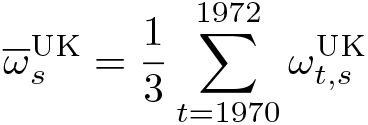
Suppose that the treated country is the United Kingdom (UK), with treatment starting in 1973. Assume that the pretreatment period is 1970, 1971, 1972 and that the post- treatment period is 1973, 1974, 1975. Suppose we use three countries as donors: France (FRA), Italy (ITA), and Germany (GER), using a set of M covariates, x = x ₁ , x ₂ ,…, x_M , for each country.

We define a distance metric based on x between each pair of countries in each year. For instance, with only one covariate x (that is, M = 1), the distance between UK and ITA in terms of x in 1970 is

d_{1970} (U K, I T A) = | | x_{1970, U K} - x_{1970, I T A} | |

Given a distance definition, the pretreatment weight for ITA will be

ω_{1970, ITA}^{UK} (h) = K (\frac{| | x_{1970} {_{,}}_{UK} - x_{1970} {_{,}}_{ITA} | |}{h})

where K(·) is a specific kernel function, h the bandwidth chosen by the analyst, and ||·|| a specific norm. The kernel function defines a weighting scheme penalizing countries that are far away from the UK and giving more relevance to countries closer to the UK. Observe that closeness is measured in terms of a predefined x distance (such as the Mahalanobis, Euclidean (L2), or modular) within a normed vector space.

Based on the chosen vector distance defined over the covariates x, we can derive the vector of weights W, whose generic element is

ω_{t, s}^{j} (h) = K (\frac{| | x_{t, j} - x_{t, s} | |}{h}) (1)

where, in this example, j = UK and s = FRA, ITA, GER.

Figure 1 provides a graphical and intuitive representation of (1). Once one has set a bandwidth h, each country in each year obtains a weight decreasing with the increasing distance from the UK. In this illustrative example, ITA gets a positive value because its distance from the UK is smaller than h; GER, on the contrary, gets a weight equal to zero because its distance from the UK is larger than h. Of course, the UK itself obtains the largest weight by default.

Figure 1.

Kernel weights representation

Following this simple example, we can define the weighting matrix W as

\begin{array}{l} \begin{matrix} 1970 & 1971 & 1972 \end{matrix} \\ W = \begin{matrix} FRA \\ ITA \\ GER \end{matrix} (\begin{array}{l} \begin{matrix} ω_{11}^{UK} & ω_{12}^{UK} & ω_{13}^{UK} \end{matrix} \\ \begin{matrix} ω_{21}^{UK} & ω_{22}^{UK} & ω_{23}^{UK} \end{matrix} \\ \begin{matrix} ω_{31}^{UK} & ω_{32}^{UK} & ω_{33}^{UK} \end{matrix} \end{array}) \end{array}

One issue is that we need just one single vector of weights, while the previous procedure provides a vector of weights for each pretreatment year. We can overcome this minor problem by taking the mean (or the median) of the yearly weights, thus defining the following augmented weighting matrix,

\begin{array}{l} \begin{matrix} 1970 & 1971 & 1972 & \begin{matrix} 1973 & 1974 & 1975 \end{matrix} \end{matrix} \\ W^{*} = \begin{matrix} FRA \\ ITA \\ GER \end{matrix} (\begin{matrix} ϖ_{FRA}^{UK} & ϖ_{FRA}^{UK} & ϖ_{FRA}^{UK} & ϖ_{FRA}^{UK} & ϖ_{FRA}^{UK} & ϖ_{FRA}^{UK} \\ ϖ_{ITA}^{UK} & ϖ_{ITA}^{UK} & ϖ_{ITA}^{UK} & ϖ_{ITA}^{UK} & ϖ_{ITA}^{UK} & ϖ_{ITA}^{UK} \\ ϖ_{GER}^{UK} & ϖ_{GER}^{UK} & ϖ_{GER}^{UK} & ϖ_{GER}^{UK} & ϖ_{GER}^{UK} & ϖ_{GER}^{UK} \end{matrix}) \end{array}

where

ϖ_{S}^{UK} = \frac{1}{3} \sum_{t = 1970}^{1972} ω_{t,s}^{UK}

Define the matrix of outcomes Y as follows (where y is the outcome):

\begin{array}{l} \begin{matrix} FRA & ITA & GER \end{matrix} \\ Y = \begin{matrix} \begin{matrix} 1970 \\ 1971 \end{matrix} \\ 1972 \\ \begin{matrix} \begin{matrix} 1973 \\ 1974 \end{matrix} \\ 1975 \end{matrix} \end{matrix} (\begin{matrix} y_{11} & y_{12} & y_{13} \\ y_{21} & y_{22} & y_{23} \\ y_{31} & y_{32} & y_{33} \\ y_{41} & y_{42} & y_{43} \\ y_{51} & y_{52} & y_{53} \\ y_{61} & y_{62} & y_{63} \end{matrix}) \end{array}

We can define a matrix C as

\underset{T \times T}{\underset{︸}{C}} = \underset{T \times J}{\underset{︸}{Y}} \times \underset{J \times T}{\underset{︸}{W^{*}}}

The diagonal of matrix C contains the “UK synthetic time series Y ₀”:

Y_{0, UK} = diag (C)

This vector is an estimation of the unknown counterfactual behavior of the UK. The generic element of the diagonal of C is

c_{t} = \underset{1 \times J}{\underset{︸}{y_{t}}} \times \underset{J \times 1}{\underset{︸}{{\bar{w}}^{*}}}

In the previous example,

c_{75}^{UK} = [y_{75} {,FRA, y}_{75} {,ITA, y}_{75},GER] \times [\begin{matrix} ϖ_{FRA}^{UK} \\ ϖ_{ITA}^{UK} \\ ϖ_{GER}^{UK} \end{matrix}] = \sum_{s = FRA,ITA,GER} y_{75},_{s} ϖ_{s}^{UK}

Therefore, c_t —that is, the synthetic outcome of the UK—is a weighted mean of controls’ y at time t, with weights provided by the previous procedure.

Previous estimation of the synthetic counterfactual is based on a specific choice of the bandwidth h. Thus, one question is how to select such bandwidth properly. As usual with nonparametric estimators, a cross-validation approach can be used (Li and Racine 2004). In this context, it reduces to select the optimal bandwidth as the one minimizing as loss objective function the preintervention root mean-squared prediction error (RMSPE) defined as

R M S P E_{j} (h) = \sqrt{\frac{1}{T_{- 0}} \sum_{t = 1}^{T - 0} {y_{j, t} - y_{j, t}^{*} (h)}^{2}}

where T ₋ ₀ is the last pretreatment time. We can estimate the optimal bandwidth computationally by first forming a grid of possible values for h and then finding h ^∗ as the value of the bandwidth minimizing the RMSPE over the grid. We provide an application of such a procedure in the next section.

4 The npsynth command

This section provides the documentation of the command npsynth, which can be used to fit the model presented in this article.

4.1 Syntax

outcome is the target variable over which one measures the impact of the treatment. varlist is the set of covariates (or observable confounding) predicting the outcome in the pretreatment period.

4.2 Description

npsynth extends the SCM for program evaluation proposed by Abadie and Gardeazabal (2003) and Abadie, Diamond, and Hainmueller (2010) to the case of a nonparametric identification of the synthetic (or counterfactual) time pattern of a treated unit. The model assumes that the treated unit—such as a country, a region, a city—underwent a specific intervention in a given year and estimates its counterfactual time pattern, the one without intervention, as a weighted linear combination of control units based on the predictors of the outcome. The nonparametric imputation of the counterfactual is computed using weights proportional to the vector distance between the treated unit’s and the controls’ predictors, using a kernel function with prefixed bandwidth. The command provides a graphical representation of the results for validation purposes.

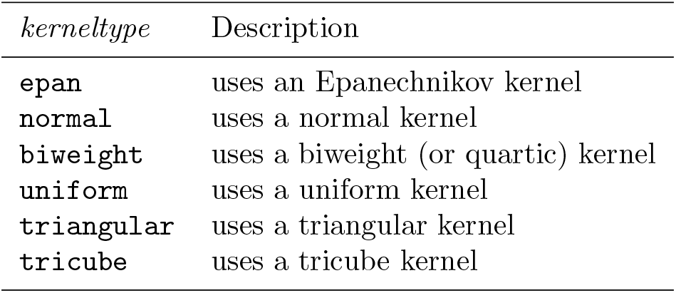
4.3 Options

trperiod( # ) specifies the time in which treatment starts. trperiod() is required.

bandw( # ) specifies the bandwidth of the kernel weighting function. bandw() is required.

panel_var( varname ) specifies the panel variable. panel_var() is required.

time_var( varname ) specifies the time variable. time_var() is required.

trunit( # ) specifies the treated unit, with # indicating one of the values taken by

panel_var(). trunit() is required.

kern( kerneltype ) specifies the type of kernel function to use for building synthetic weights. kern() is required.

npscv allows for computing the optimal bandwidth minimizing the pretreatment RMSPE. The default length of the grid over which to find the optimal bandwidth is 20, which means that the bandwidth’s grid is [0.1, 0.2,…, 2]. This option returns the optimal bandwidth in the e-class object e(opt_band).

n_grid( #1 , #2 ) specifies the length of the grid over which to find the optimal bandwidth. The default is n_grid(1, 20), which means that the bandwidth’s grid is [0.1, 0.2,…, 2].

save_res( filename ) saves the treated factual and counterfactual time patterns in filename .dta.

w_median specifies that the unique vector of synthetic weights be calculated by the yearly weight’s median (the default uses the mean).

gr_y_name( name ) gives a convenient name to the outcome variable to appear in the graphs.

gr_tick( # ) sets the tick of the time in the time axis of the graphs.

gr1 plots the pretreatment balancing and parallel trend graph.

gr2 plots the overall treated and synthetic-pattern comparison graph.

gr3 plots the overall pattern of the difference between the treated and synthetic-pattern graph.

save_gr1( graphname1 ) saves graph 1, that is, the pretreatment balancing and parallel trend.

save_gr2(graphname2) saves graph 2, that is, the overall treated and synthetic-pattern comparison.

save_gr3( graphname3 ) saves graph 3, that is, the overall pattern of the difference between the treated and synthetic pattern.

4.4 Stored results

npsynth stores the following in e():

4.5 Requirements

Before running npsynth, one must first install the moremata (Jann 2005) and mahapick (Kantor 2006) packages. npsynth uses the command mahascore from the mahapick package.

Finally, cross-validation optimal bandwidth can be obtained using the npsynth‘s postestimation command npscv, which returns the optimal bandwidth via the return scalar e(opt_band). The command npscv takes neither arguments nor options; thus, it can be easily typed immediately after running npsynth. The command also provides a graphical representation of the RMSPE minimization.

5 Simulation

Before presenting an application on real data, I perform a simulation example to show how npsynth improves counterfactual estimation precision compared with the traditional SCM (estimated by the command synth) when nonlinearities are considered.

I perform an SCM simulation using a data-generating process (DGP) where E(x ₁|X ₀), that is, the projection of the covariates of the treated unit over the vector space spanned by the covariates of the donors, is highly nonlinear. This contrasts with the linearity assumption of this projection used by the Abadie, Diamond, and Hainmueller (2010) model, while it should suitably accommodate the nonlinear projection used by npsynth.

Because the simulation code is pretty long, for the sake of brevity, I do not report the code here. One can reproduce it by running the do-file simulation_npsynth.do. Thus, I focus on the main DGP assumptions and related results.

We consider a setting with three normally distributed covariates x ₁ , x ₂ , x ₃, one treated unit, and three donors {1, 2, 3}. We model the three covariates for the treated unit in a highly nonlinear way as a function of the respective covariates of the three donors,

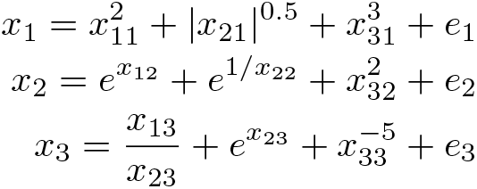
\begin{array}{l} x_{1} = x^{2}_{11} + | x_{21} |^{0} {^{.}}^{5} + x^{3}_{31} + e_{1} \\ x_{2} = e^{x} 12 + e^{1}^{/ x} 22 + x^{2}_{32} + e_{2} \\ x_{3} = \frac{x_{13}}{x_{23}} + e^{x_{23}} + x_{33}^{- 5} + e_{3} \end{array}

where e_i are normally distributed errors. This specification of E(x ₁|X ₀) is thus far from the linear one implied by synth. The observed (or factual) outcome of the treated unit is

y_{1} = x_{1} + x_{2} + x_{3} + e

while the counterfactual is

y_{0} = {\begin{cases} x^{1} + x^{2} + x^{3} + e if t \leq 2009 \\ - 100 + x_{1} + x_{2}^{0.7} + log (| x 3 |) + e if t > 2009 \end{cases}

where the year of treatment is 2009. Figure 2 sets out the plot of the factual and counterfactual pattern of the treated unit according to the above specified DGP.

Figure 2.

Simulated factual and counterfactual pattern of the treated unit outcome when the policy occurs at year 2009

Also, we generate the donors’ pattern as the counterfactual pattern of the treated units plus a normally distributed shock with different means and variances. Results are plotted in figure 3.

Figure 3.

Simulated treated and donors outcome pattern, when policy occurs in year 2009

We apply both synth and npsynth to this simulated dataset. Figure 4 shows the plots of the DGP counterfactual outcome (the true one) and the ones estimated by synth and npsynth.

Figure 4.

Estimated counterfactual: Comparison between npsynth and synth; policy occurs in year 2009

As expected, results show that npsynth substantially outperforms synth, especially in year 2012, 2013, and 2015. Importantly, the synth‘s RMSPE is equal to 8.96 against a lower value of 6.65 achieved by npsynth. Notice also that, in terms of mean squared prediction error, the npsynth error is half the one provided by synth. This lends support to the main idea of this article, that is, that the linearity restriction does matter in the construction of the synthetic counterfactual.

6 Application

In this section, I compare the proposed nonparametric approach and the parametric approach provided by Abadie, Diamond, and Hainmueller (2010) by focusing on the effects of adopting the Euro as the national currency. In 2001, some European countries abandoned their national currencies to adopt the Euro. It is thus interesting to understand whether this relevant institutional change has had an impact on European economies. Of course, one can consider many outcome variables over which to measure such an effect. In this exercise, we focus on one specific country, Italy, and one specific outcome, namely, the domestic direct value added (DDVA) exports obtained by using the gross export decomposition suggested by Wang, Wei, and Zhu (2013).

To evaluate the goodness of fit of both procedures, we consider the preintervention RMSPE for Italy (that is, the average of the squared discrepancies between DDVA in Italy and in its synthetic counterpart during the pretreatment period). As donors, we consider a set of 18 countries worldwide that experienced no change in currency adoption during the period under scrutiny. In this case, the RMSPE formula is

{RMSPE}_{ITA} = \sqrt{\frac{1}{T_{- 0}}} \sum_{t = 1}^{T - 0} {(y_{t, ITA} - y_{t}^{*},_{ITA})}^{2}

with T ₋ ₀ = 1999. We consider 2000 as the year of treatment because many transactions were done using the Euro starting from one year before the currency was officially adopted.

The model specification is a type of gravity model, which is standard in the economics of trade, taking as explanatory variables the same DDVA, the log of the distance between each pair of countries, the sum of their GDP, the presence of a common language, and a contiguity measure between countries.

By applying the Abadie, Diamond, and Hainmueller (2010) model to this dataset and specification, we obtain the following results:

The RMSPE is equal to 0.008, which is quite small. The donors’ optimal weights, as reported above, show that only four countries are used as donors: Great Britain, Japan, Poland, and Sweden. The largest weight is the one of Poland, with a value of around 0.6, followed by that of Japan (0.18), and Great Britain (0.12). The subsequent panel, finally, shows that all the predictors are sufficiently balanced, thus entailing a good quality in the construction of the pretreatment synthetic counterfactual.

The good performance provided by the Abadie, Diamond, and Hainmueller (2010) method is confirmed by figure 5, plotting over the years the treated and synthetic pattern of the outcome variable DDVA. This figure clearly shows an effect of adopting the Euro, because after 2000, the synthetic and treated patterns diverge considerably. In particular, it seems that in the absence of the Euro, the DDVA would have been lower than that experienced in adopting the Euro. This means that the Euro seems to have had positive effects in increasing the DDVA component of the gross export for Italy.

Figure 5.

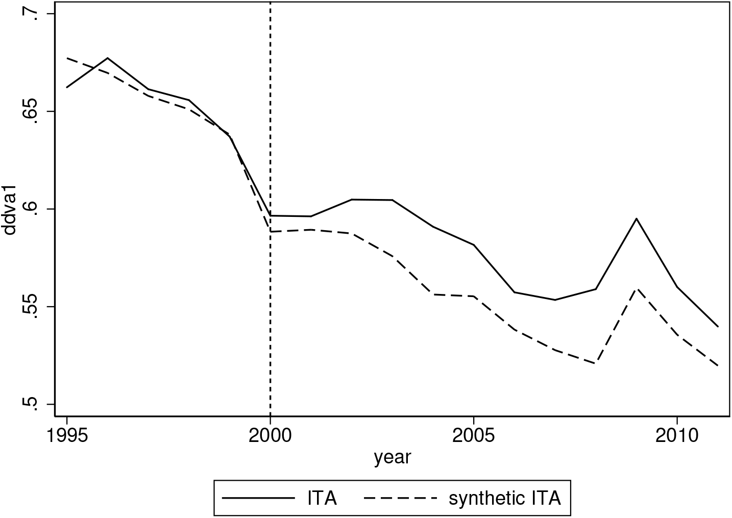
Treated and synthetic pattern of the outcome variable DDVA. Parametric model.

When applying the nonparametric approach proposed here, one has to first find the optimal bandwidth. As said, we select the bandwidth by minimizing the RMSPE. Results are reported in figure 6, where we can see that the RMSPE is minimized at a bandwidth equal to 0.5. Both the optimal bandwidth and the graph in the figure can be obtained by inserting the option npscv into the npsynth command as we set out below.

Figure 6.

Optimal bandwidth by minimizing the RMSPE

A graphical inspection, however, shows that a bandwidth equal to 0.4 (namely, a slight undersmoothing) performs better for years closer to the treatment year, thus making it more appropriate to use such a bandwidth as the optimal one in the estimation of the synthetic pattern. The panel of results below sets out that the value of the RMSPE is 0.01, a bit larger than that found in the parametric case. Also, the weighting scheme is different, with more donors having a nonzero weight, and China obtaining the lion’s share.

The graph in figure 7 shows a good fit of the model, which slightly outperforms the parametric method when gradually approaching the treatment time. This improvement is not signaled by overall RMSPE, because the nonparametric estimation performs worse than the parametric one at the very beginning of the pretreatment period, which is less relevant, however, for assessing the overall quality of the fit. To assess that npsynth provides a smaller RMSPE close to the time of treatment (year 2000), we rerun both models and estimate the pretreatment fit considering only the years between 1996 and 2000 via this supplementary code:

Figure 7.

Treated and synthetic pattern of the outcome variable DDVA. Nonparametric model.

In this case, we can see that the nonparametric approach behaves a bit better than the parametric one (with a RMSPE of 0.0034 against 0.0048), although both provide a small pretreatment prediction error.

7 Conclusions

This article has provided an extension of the SCM for program evaluation to the case of a nonparametric identification of the synthetic (or counterfactual) time pattern of a treated unit. After briefly presenting the parametric method, I introduced the nonparametric alternative by focusing on npsynth, which I used to implement the nonparametric SCM. I proposed a parametric versus nonparametric comparative assessment both on simulated and real data. Both exercises showed that, while both methods provide a small pretreatment prediction error, the nonparametric approach tends to outperform the parametric one, especially in the presence of high nonlinearity in the relationship between the treated unit’s and the donors’ covariates.

The novel approach herein proposed can thus complement the traditional one by providing more robustness to program evaluation results obtained using the SCM.

Supplemental Material

Supplemental Material, st0619 - Nonparametric synthetic control using the npsynth command

Supplemental Material, st0619 for Nonparametric synthetic control using the npsynth command by Giovanni Cerulli in The Stata Journal

Footnotes

8 Acknowledgments

I thank the organizers of and participants in the 23rd London Stata Conference, held on the 7–8 September 2017 at Cass Business School (London, UK), where a preliminary version of this article was presented. In particular, I thank Kit Baum for the careful reading of this article.

9 Programs and supplemental materials

To install a snapshot of the corresponding software files as they existed at the time of publication of this article, type

This routine is freely downloadable from the Stata Statistical Software Components archive,

. ssc install npsynth

Notes

References

Abadie

Diamond

Hainmueller

. 2010. Synthetic control methods for comparative case studies: Estimating the effect of California’s tobacco control program. Journal of the American Statistical Association 105: 493–505. https://doi.org/10.1198/jasa.2009.ap08746.

Abadie

Gardeazabal

. 2003. The economic costs of conflict: A case study of the Basque country. American Economic Review 93: 113–132. https://doi.org/10.1257/000282803321455188.

Abadie

L’Hour

. 2019. A penalized synthetic control estimator for disaggregated data. https://sites.google.com/site/jeremylhour/research.

Angrist

J. D.

Pischke

J.-S.

. 2009. Mostly Harmless Econometrics: An Empiricist’s Companion. Princeton, NJ: Princeton University Press.

Angrist

J. D.

Pischke

J.-S.

. 2010. The credibility revolution in empirical economics: How better research design is taking the con out of econometrics. Journal of Economic Perspectives 24: 3–30. https://doi.org/10.1257/jep.24.2.3.

Autor

D. H.

2003. Outsourcing at will: The contribution of unjust dismissal doctrine to the growth of employment outsourcing. Journal of Labor Economics 21: 1–42. https://doi.org/10.1086/344122.

Card

Krueger

A. B.

. 1994. Minimum wages and employment: A case study of the fast-food industry in New Jersey and Pennsylvania. American Economic Review

Cerulli

2015. Econometric Evaluation of Socio-Economic Programs: Theory and Applications. Berlin: Springer.

Cerulli

2019. A flexible synthetic control method for modeling policy evaluation. Economics Letters 182: 40–44. https://doi.org/10.1016/j.econlet.2019.05.019.

10.

Hastie

Tibshirani

Friedman

. 2009. The Elements of Statistical Learning: Data Mining, Inference, and Prediction. 2nd ed. New York: Springer.

11.

Imbens

G. W.

Rubin

D. B.

. 2015. Causal Inference for Statistics, Social, and Biomedical Sciences: An Introduction. New York: Cambridge University Press.

12.

Jann

2005. moremata: Stata module (Mata) to provide various functions. Statistical Software Components S455001, Department of Economics, Boston College. https://ideas.repec.org/c/boc/bocode/s455001.html.

13.

Kantor

2006. mahapick: Stata module to select matching observations based on a Mahalanobis distance measure. Statistical Software Components S456703, Department of Economics, Boston College. https://ideas.repec.org/c/boc/bocode/s456703.html.

14.

Racine

. 2004. Cross-validated local linear nonparametric regression. Statistica Sinica 14: 485–512.

15.

Racine

J. S.

. 2007. Nonparametric Econometrics: Theory and Practice. Princeton, NJ: Princeton University Press.

16.

Pagan

Ullah

. 1999. Nonparametric Econometrics. Cambridge: Cambridge University Press.

17.

Wang

Wei

S.-J.

Zhu

. 2013. Quantifying international production sharing at the bilateral and sector levels. NBER Working Paper No. 19677, The National Bureau of Economic Research. https://www.nber.org/papers/w19677.

Supplementary Material

Please find the following supplemental material available below.

For Open Access articles published under a Creative Commons License, all supplemental material carries the same license as the article it is associated with.

For non-Open Access articles published, all supplemental material carries a non-exclusive license, and permission requests for re-use of supplemental material or any part of supplemental material shall be sent directly to the copyright owner as specified in the copyright notice associated with the article.

0.01 MB

0.00 MB