merlin—A unified modeling framework for data analysis and methods development in Stata

Abstract

The challenges in statistics and data science are rapidly growing because access to a multitude of data types continues to increase, as well as the sheer quantity of data. Analysts are now presented with multivariate data, sometimes measured repeatedly, and often requiring the ability to model nonlinear relationships and hierarchical structures. In this article, I present the merlin command, which attempts to provide an extremely general framework for data analysis. From simple settings such as fitting a linear regression model or a Weibull survival model to more complex settings such as fitting a three-level logistic mixed-effects model or a multivariate joint model of multiple longitudinal outcomes (of different types) and a recurrent event and survival with nonlinear effects, merlin can fit them all. I will take a single dataset and attempt to show you the full range of capabilities of merlin and discuss some future directions for the implementation in Stata.

1 Introduction

gsem‘s introduction in Stata 14 brought an extremely broad class of mixed-effects models (among other things); most importantly (from my perspective), gsem is fast. gsem has full analytic derivatives for any model that you fit, including a model with any number of levels and random effects at each level. Of course, gllamm preceded gsem, providing a very flexible framework in Stata for modeling data (Rabe-Hesketh, Skrondal, and Pickles 2002, 2005). But inevitably, every program is limited to certain families of distributions, complexity of the linear predictors, and of course computational speed. There is also the widely used community-contributed cmp package by Roodman (2011), which implements joint modeling of multivariate processes, assuming joint normality. Bartus (2017) further demonstrated gsem‘s capabilities in modeling simultaneous equation systems, including multilevel hazard equations with correlated random effects, with a focus on piecewise exponential models. merlin builds directly on these works but focuses on more flexible parametric distributions, extending linking between outcome models, and nonlinear modeling capabilities.

Much of my previous work has centered on joint longitudinal survival analysis, implemented in the stjm command (Crowther, Abrams, and Lambert 2013), which can fit a joint model for a continuous, repeatedly measured biomarker and a single time to event. There is flexibility in that you can use splines or polynomials to model the biomarker over time, and there are lots of choices for your survival model, including spline-based approaches. The main benefit of stjm is the added flexibility in how to link the two submodels through things such as the expected value, or derivatives of it, which are commonly used in the joint model literature. Given this starting point, the natural extension is to allow for more than one biomarker, recurrent events, competing risks, etc. I have also released stmixed (Crowther, Look, and Riley 2014) for two-level parametric survival models, in particular for the Royston–Parmar spline-based model, and stgenreg for general hazard-based regression (Crowther and Lambert 2013, 2014), where users could specify their own functional form for the hazard function and stgenreg would use numerical quadrature to calculate the likelihood.

The aim of merlin is not only to bring together my previous programs but also to provide a whole lot more. In this article, I will introduce the core features and syntax of merlin and illustrate a variety of models that can be fit with it. More details on the methodological framework can be found in Crowther (2017). The article is structured as follows: In section 2, I describe the top-level syntax of the merlin command and describe many of the options. In section 3, I detail many examples, showing the wide variety of available models. In section 4, I conclude the article with a discussion of merlin and its potential.

2 The architecture of merlin

merlin is designed to be as flexible and general as possible. There is no real limit to what it can do, given that the user can readily extend it. You can specify any number of outcome models, which can be linked in any number of ways. Each outcome model, i = 1,…, M, has a main complex predictor (you can have more, but I will leave that for another time) that comprises additive components, c = 1,…, C_i , where each component comprises multiplicative elements, e = 1,…, E_ic ,

$g_i\left\{{\mu }_i\left(y_i|x,b\right)\right\}={\displaystyle \sum _{c=1}^{C_i}{\displaystyle \prod _{e=1}^{E_{ic}}{\psi }_{ice}}}\left(x,b\right)$

where for the ith model, y_i is the observed response, x is the full-design matrix, and b are the stacked multivariate normal or t distributed random effects. We have link function g_i (·) and expected value µ_i . ψ(·) defines essentially an arbitrary function, of which some special cases are defined in the next section.merlin models are fit using maximum likelihood, with any random effects integrated out using adaptive or nonadaptive Gaussian quadrature or Monte Carlo integration.

More details on the formulation of the likelihood can be found in Crowther (2017) or the Stata manual entry for gsem because the formulation and default integration options (adaptive Gauss–Hermite quadrature) are the same.

2.1 merlin syntax

merlin ( model1) [( model2)] […] [ if] [in] [, options]

where the syntax of a model is

[depvar] [component1] [component2] […] [if] [in] [, model options]

where the syntax of a component is

element1 [#element2] [#element3] […] [@ real]

and each elementk can take one of the forms described in the next section. At the end of each component, you may optionally specify a constraint on the parameter or parameters of the associated component by using @.

model_options include the following:

family( family , fam_options ), where family can be one of

– gaussian—Gaussian distribution

– bernoulli—Bernoulli distribution

– beta—beta distribution

– poisson—Poisson distribution

– ologit—ordinal with logistic link

– oprobit—ordinal with probit link

– gamma—gamma distribution

– exponential—exponential distribution

– gompertz—Gompertz distribution

– rp—Royston–Parmar model (restricted cubic spline on log cumulative-hazard scale)

– loghazard—general log-hazard model

– logchazard—general log cumulative-hazard model

– weibull—Weibull distribution

– user—specify your own distribution

and fam_options include the following:

– failure( varname )—event indicator for a survival model

– ltruncated( varname )—left-truncation/delayed entry times for survival model

– llfunction( func_name )—name of a Mata function that returns your user-defined log-likelihood contribution

– hfunction( func_name )—name of a Mata function that returns your user-defined hazard function

– chfunction( func_name )—name of a Mata function that returns your user-defined cumulative hazard function

– nap( # )—estimate # ancillary parameters, which may be called in user-defined functions

timevar( varname ) specifies the variable that contains time; this is required to specify time-dependent effects. Generally, within a survival model, time must be explicitly handled by merlin. timevar() will be matched against any elements (see the next section) that may use it to make sure it is handled correctly.

There are many other suboptions available in merlin, which are fully documented in the help files.

Element types

One of the fundamental flexibilities of merlin is the variety of elements that can be used within your model.

varname is an independent variable in your dataset.

rcs( varname , opts ) is a restricted cubic spline function, where opts include the following:

– df( # ) is degrees of freedom (# of internal knots + 1). Knots are placed at evenly spaced centiles of varname, with boundary knots assumed to be the minimum and maximum of varname.

– knots( knots_list ) specifies the knots, including the boundary knots.

– orthog applies Gram–Schmidt orthogonalization, which can improve convergence.

– event used in conjunction with df() specifies that internal knot locations be based on centiles of only observations of varname that experienced the survival event specified in failure().

– log creates splines of log( varname ) instead of the default untransformed varname.

– offset( varname ) specifies an offset to be added to varname before the rcs() function is built.

bs( varname , opts ) is a B-spline function, where opts include the following:

– df( # ) specifies the degrees of freedom (not strictly speaking) for the spline function, which allows you to specify internal knots at equally spaced centiles, instead of using

– knots(). df() is consistent with rcs() elements in how internal knots are chosen.

– knots( knots_list ) specifies the internal knots. They must be in ascending order.

– bknots( knots_list ) specifies the lower- and upper-boundary knot locations. They must be in ascending order. The default is the minimum and maximum of varname.

– event used in conjunction with df() specifies that internal knot locations be based on centiles of only observations of varname that experienced the survival event specified in failure().

– log creates splines of log( varname ) instead of the default untransformed varname.

– intercept includes the intercept basis function, which by default is not included.

– offset( varname ) specifies an offset to be added to varname before the bs() function is built.

fp( varname , opts ) is a fractional polynomial function (of order 1 or 2), where opts include the following:

– powers( numlist ) powers up to a second-degree fractional polynomial function, each of which can be one of (−2, −1, −0.5, 0, 0.5, 1, 2, 3).

– offset( varname ) specifies an offset to be added to varname before the fp() function is built.

mf( function_name ) is a user-defined Mata function.

M # [ cluster_level ] is a random effect defined at the cluster_level; for example, M1[centre] defines a random intercept at the centre level, and M2[centre>id] defines a random intercept at the id level.

EV[ depvar | # ] is the expected value of an outcome model.

dEV[ depvar | # ] is the first derivative with respect to time of the expected value of an outcome model.

d2EV[ depvar | # ] is the second derivative with respect to time of the expected value of an outcome model.

iEV[ depvar | # ] is the integral with respect to time of the expected value of an outcome model.

XB[ depvar | # ] is the expected value of a complex predictor.

dXB[ depvar | # ] is the first derivative with respect to time of the expected value of a complex predictor.

d2XB[ depvar | # ] is the second derivative with respect to time of the expected value of a complex predictor.

iXB[ depvar | # ] is the integral with respect to time of the expected value of a complex predictor.

merlin postestimation

merlin comes with a set of postestimation tools available through the predict function, with the standard syntax of predict newvar [, statistic options]

where statistic includes the following:

mu—expected value of the response

eta—expected value of the complex predictor

survival—survival function

cif—cumulative incidence function

hazard—hazard function

chazard—cumulative hazard function

rmst—restricted mean survival time (integral of survival)

timelost—time lost because of the event (integral of cif)

totaltimelost—total time lost because of all events, within (0, t]

mudifference—differences in expected values of depvar

etadifference—differences in expected value of complex predictor

hdifference—differences in hazard functions

sdifference—differences in survival functions

cifdifference—differences in cumulative incidence functions

rmstdifference—differences in restricted mean survival functions

options include the following:

fixedonly calculates prediction based only on the fixed effects.

marginal calculates prediction integrating out all random effects, that is, the population-averaged prediction.

outcome( # ) specifies the model to predict for; the default is outcome(1).

causes( numlist ) specifies which models contribute to the calculation; this is for use in competing risks models.

at( at_spec ) specifies covariate patterns at which to calculate statistic, for example, at(trt 1 age 54).

ci calculates confidence intervals using the delta method through predictnl.

timevar( varname ) specifies a variable that contains time points at which to calculate statistic.

at1( at_spec ) specifies covariate values for the first contrast.

at2( at_spec ) specifies covariate values for the second contrast.

intpoints( # ) uses # integration points to compute marginal predictions.

3 Examples

Given how varied and complex the syntax can appear, the easiest way to get to grips with merlin is through some examples. Throughout this section, I will use a single dataset (Murtaugh et al. 1994). It is a commonly used dataset from the joint longitudinal survival literature and will serve to illustrate many different analysis techniques, culminating in a detailed, complex multivariate hierarchical model. First, I load the data, which you can get from my website,

. use "https://www.mjcrowther.co.uk/data/jm_example" (Example dataset for joint modelling, Michael Crowther 2011)

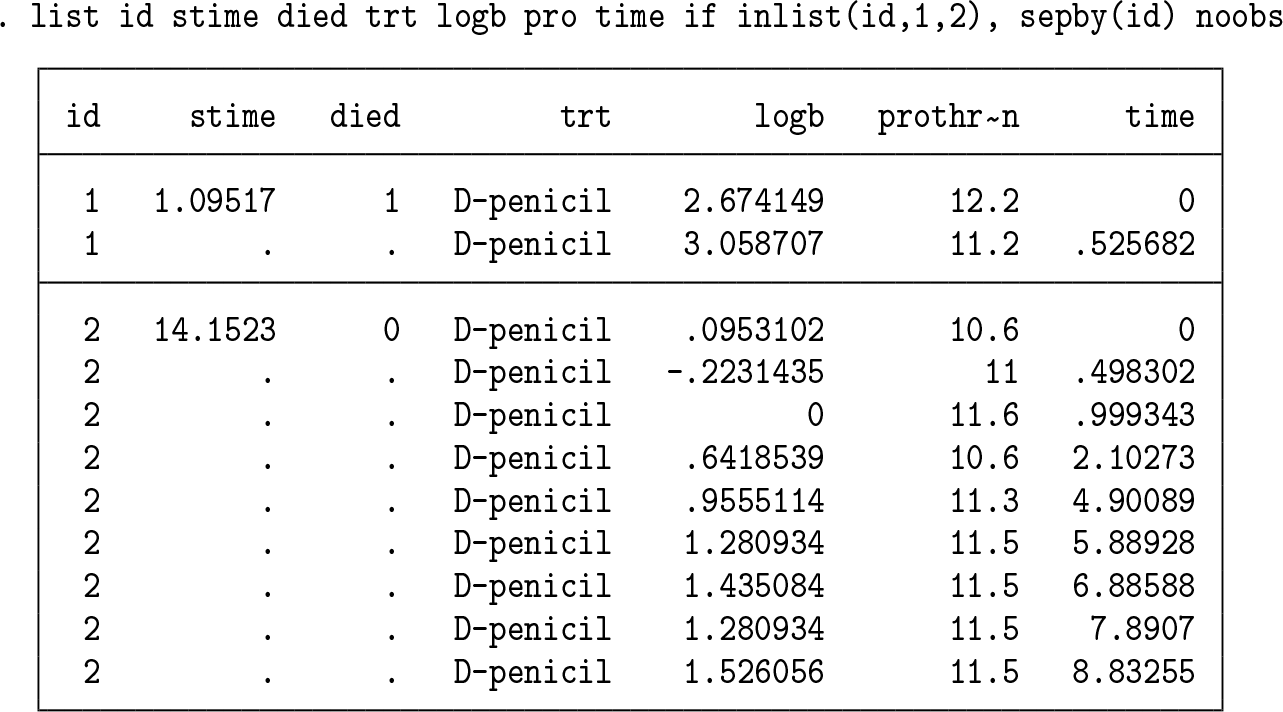
The dataset consists of information on 312 patients with primary biliary cirrhosis, of which 140 died during a maximum follow-up of 14.3 years. Covariates of interest include serum bilirubin and prothrombin index, both markers of liver performance, and treatment allocation, trt. Patients were randomized to either D-penicillamine or a placebo. In all analyses, I will work with the log of serum bilirubin, stored in logb. The data structure looks as follows:

merlin, just like gsem, treats models in wide format but observations within a model in long format. Hence, our survival outcome variables, stime and died, must have only one observation per id. If a patient had more than one row of data for his or her survival outcome, then we could fit a recurrent event model. The time variable records the times at which the biomarkers logb and prothrombin were recorded.

3.1 Linear mixed-effects regression

I will start with a very simple model, a linear regression of logb against time, assuming a Gaussian response:

Let’s add some flexibility by using the rcs() element, which lets us model the change over time flexibly using restricted cubic splines with three degrees of freedom, that is, three spline terms.

If you prefer fractional polynomials or B-splines, then use the fp() or bs() element types. Given our observations are clustered within individuals, let’s add a random intercept:

I have added M1[id]@1 to my complex predictor. This defines a single normally distributed random effect, called M1, defined at the id level. By default, any component within the complex predictor will have an estimated coefficient. Given our model will already estimate a fixed intercept, we want to constrain the random-effects coefficient to be 1 by specifying @1 at the end. Let’s add a random linear slope and also orthogonalize my spline terms:

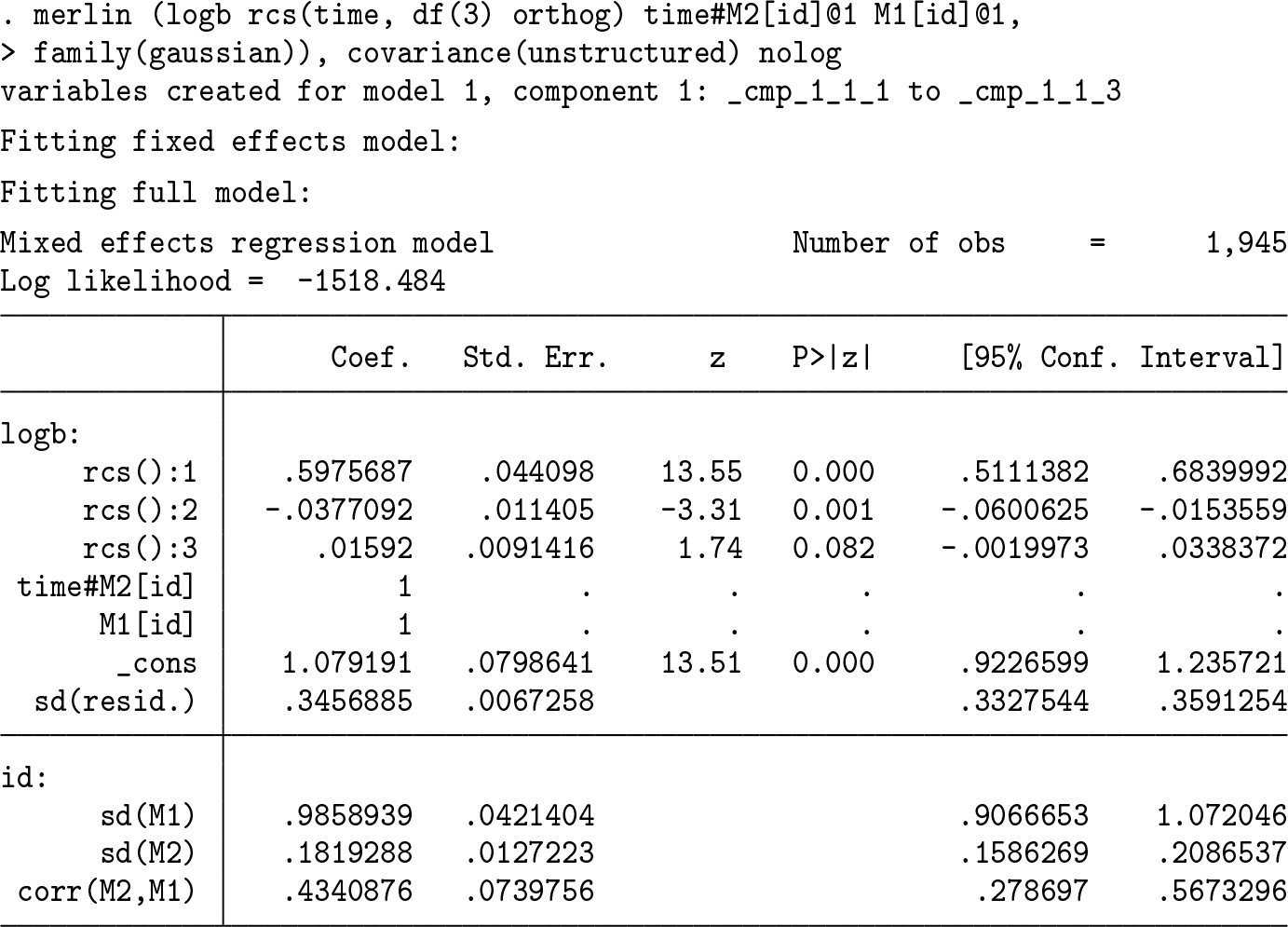
Note by orthogonalizing the splines, we change the interpretation of the intercept. I now have a component with more than one element, time#M2[id]@1—a variable time has been multiplied by a random effect called M2 defined at the id level, with its coefficient constrained to be 1. If I called it M1 again, then there would only be a single random effect in my model but used twice, which would not be sensible in this case. By default, each level’s random effects are assumed to have covariance(diagonal). We can relax this by estimating a correlation,

Estimating the correlation shows evidence of positive correlation between intercept and slope.

3.2 Survival and time-to-event analysis

Many standard time-to-event models are available in merlin, including most of those in streg, and some more flexible distributions are also built in. This includes the Royston–Parmar model and a log-hazard scale equivalent model, both using restricted cubic splines to model the baseline. To fit a survival model with merlin, we simply add the failure() option to specify the event indicator.

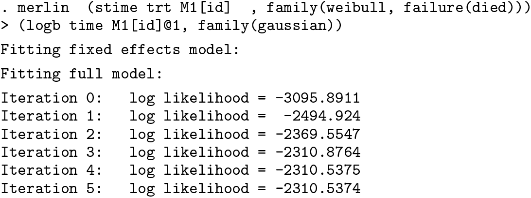
Weibull proportional hazards model

Let’s start with a simple Weibull proportional hazards model, adjusting for treatment, with all parameters estimated on the log scale.

Spline-based survival model

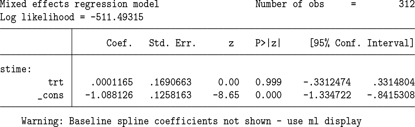
The Royston–Parmar model is now widely used, using restricted cubic splines to model the baseline log cumulative-hazard function and any time-dependent effects:

I model the baseline with 3 spline terms using the df() option. Note the spline coefficients are not shown by default (they are essentially uninterpretable). You can show all the parameters by using ml display.

Assess proportional hazards

Let’s assess proportional hazards in the effect of treatment by forming an interaction between treatment and log time:

We had to specify our timevar() so merlin knows to handle it differently. Equivalently, we could have used the rcs() element type:

Add a nonlinear effect

We can keep building this model by investigating the effect of age, modeled flexibly using fractional polynomials:

Delayed entry/left-truncation

We can allow for delayed entry/left-truncation by using the ltruncated() option. Because we have no delayed entry in this dataset, I simulate it as an illustration:

3.3 Competing risks

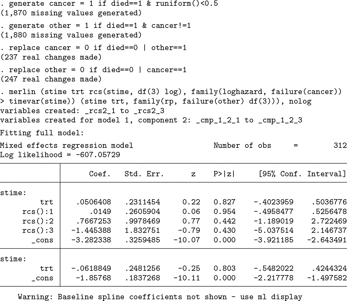
Now I will look at a multiple-outcome survival model, for example, the competing risks setting. This is done by specifying cause-specific hazard models. Remember our data structure is simplest in wide format, and within a competing risks setting, our survival time is either censoring or event time; regardless of the event, we simply need cause-specific event indicators. Because this dataset has only all-cause mortality, I randomly assign half of them to represent death from cancer, cancer, and the other half to death from other causes, other. We can then model each cause-specific hazard in any way we like, for example,

This models cause 1 with splines on the log-hazard scale and cause 2 with splines on the log cumulative-hazard scale.

Let’s calculate the cumulative incidence functions for each cause using the predict tools. I will generate a time variable and calculate the predictions for a patient in the treated group.

By default, causes() will include all models, but I am being explicit here for clarity. To create a stacked plot, we need to add the two cumulative incidence functions and then use area graphs:

Figure 1.

Stacked cumulative incidence functions

3.4 Joint modeling of longitudinal and survival data

Now I will move into the field of joint longitudinal survival models. Joint models were first proposed by linking the submodels through the random effects only, such as

By including my random intercept M1 in the complex predictor for the survival outcome, and not specifying a constraint, we will obtain an association parameter for the relationship between the subject-specific random intercept of the biomarker and survival. Alternatively, and now more commonly, we can use the EV[] element type to link the time-dependent expected value of the biomarker directly to the risk of event. Given we are modeling time, timevar() must be specified in both submodels because it will be integrated over in the survival model likelihood contribution.

There is no limit in how many associations and what form we specify; for example, we can also link the cumulative value of the biomarker (think of it as cumulative exposure) directly to survival.

Nonlinearities in the association and time-dependent effects can also be specified.

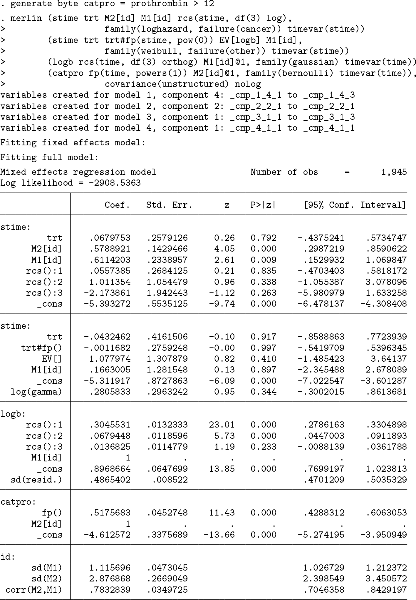
3.5 A final model

Now I am going to combine many of the previous models into one merlin model. This is purely for illustration but hopefully gives you an idea of just how flexible merlin can be. I will now generate a binary, repeatedly measured variable, catpro, that is prothrombin merely categorized into above and below 12 (this is clearly an unnecessary thing to do but purely for illustration). I will also use the artificial competing risks outcomes created above and so combine a joint model for two repeatedly measured outcomes, one continuous and one binary, with cause-specific competing risks survival models. Each cause-specific hazard model will have a different distribution, and we can allow for time-dependent effects and nonproportional hazards.

There are four outcome models and 2 random effects, so it takes some time, but we get there in about 16 minutes on my laptop. It is trivial to extend this model, for example, by adding random slopes or different ways of linking the submodels or incorporating nonlinear effects, be they for continuous covariates or time. Importantly, we can use the predict function to obtain easily understandable measures of risk, such as cumulative incidence functions, even from such a complex joint model.

4 Discussion

I have given a broad overview of merlin‘s capabilities, and potential, in the field of data analysis. I have described the fundamental syntax and, through worked examples, illustrated some of the areas of statistical modeling that can be applied using merlin.

4.1 The curse of generality

When you implement a software package that can do many things, one of the challenging tasks is to balance said generality with computational speed. merlin is not the quickest. Its current implementation is a gf0 evaluator, which means it uses Stata’s internal finite difference routines within the ml engine to calculate the score and Hessian, which means a lot of calls to the evaluator program. Furthermore, merlin has to cover many different settings and options, which inevitably means storing a lot of information within its main object. You will get speed gains if you implement a specific command, from scratch, designed for a specific setting.

4.2 Wrapper commands

First, the syntax of merlin is not the simplest. This is of course because it has to accommodate a lot of different options and techniques. This opens up more room to go wrong. Second, it is rather challenging to obtain good starting values for a command that can fit anything, and good starting values can be crucial to improve convergence.

This motivates the writing of wrapper commands, that is, ado-files specifically written to handle specific classes of merlin models. This allows a much simpler and cleaner syntax and the ability to hard-code initial-value fitting routines. Under the hood, and unbeknown to most users, the shell command will call merlin. The first of these is stmixed (Crowther 2019). I am working on a few more of these.

4.3 Concluding remarks

There is a multitude of future directions in which to take merlin. This includes adding analytic derivatives for computational speed gains, extending the allowed random-effects distributions to allow things such as mixtures of Gaussians, and providing more tools for postestimation, including dynamic prediction capabilities. In a future article, I plan to focus on the user-defined and custom distribution capabilities of merlin.

Supplemental Material

Supplemental Material, st0616 - merlin—A unified modeling framework for data analysis and methods development in Stata

Supplemental Material, st0616 for merlin—A unified modeling framework for data analysis and methods development in Stata by Michael J. Crowther in The Stata Journal