Multistate life tables using Stata

Abstract

The mslt command calculates the functions of a multistate life table and plots a graph of conditional and unconditional life expectancies by time. The command provides linear and exponential solutions to estimate the number of individuals, transitions, probabilities, person-years, and years of life in a given cohort and state of occupancy. The input data are time-specific transition rates (or survivorship proportions) between nonabsorbing and at most one absorbing state. In addition to the mean age at transfer between states, mslt calculates the following summary measures: the mean age, the probability of dying, the average duration, and the proportion of life spent in a specific state.

1 Introduction

Multistate, or increment–decrement, life tables are a demographic tool to calculate the amount of time that individuals of a cohort will spend in a given state of occupancy, broadly defined by the presence of a categorical attribute. In comparison with singlestate life tables, a unique feature of multistate tables is to decompose the overall life expectancy into segments of life span by different states, which make the analytical approach of multistate life tables applicable to many areas (Ledent and Zeng 2010). In the sociology of the family, examples of valid states for investigation are single, married, divorced, or widowed. In social stratification, one could examine the odds and the time spent in the working, middle, and upper classes. In epidemiology, the focus could be on noninfected versus infected individuals or experiencing no disability versus being disabled. In labor economics: employed, unemployed, or retired. In geography: residing in rural or urban areas. In political science: being a Democrat, a Liberal, or a Republican or having no political affiliation. Multistate life tables allow the calculation of how many years one could expect to spend in each one of these categories and provide other informative functions to understand social processes of change and composition of groups. In all these examples, an additional and ultimate absorbing state (which once entered cannot be left) could be included: death, but also unrecoverable illnesses, or physical conditions. Differently from single life tables, where death is typically the only source of exit, in multistate life tables, increments and decrements from more than one state are allowed, making it a rich analytical framework to model flows under the influence of concurrent risks.

Multistate models answer the following questions: How long could one expect to live in a given condition? What is the probability of moving from one condition to another? What is the probability of dying in a given state? At what time of exposure (that is, ages) are transitions between states of interest most likely to occur? How long can one born in a given condition expect to live in alternative states?

Once transition rates—or survivorship proportions—by time ¹ and between states are entered in Stata, mslt calculates unconditional and conditional life expectancies and optionally provides the proportion of life, the mean age of persons, the average duration, the probabilities of transition, and the mean lifetime at transfer between states. The goal of this article is to introduce and illustrate the use of mslt, a Mata-based command to calculate functions and key summary measures of multistate life tables.

2 Background

Increment–decrement life tables have a long history in demography. The oldest application dates from the early 20th century, when DuPasquier (1912) investigated transitions between two conditions: healthy and disabled. Since then, much work has been done to advance and implement multistate models (Rogers 1973, 1975; Ledent 1980; Schoen 1988a,b; Palloni 2001), with applications to marital status (Schoen and Land 1979), labor force participation (Smith 1982; Willekens 1980), interregional migration (Rogers 1975), population projections by educational attainment (Lutz and Goujon 2001), active and disabled (Land, Guralnik, and Blazer 1994), and happy life expectancies (Yang and Walij 2010). In addition, a plethora of computer programs have been written to estimate multistate life tables (Willekens and Putter 2014), but most of them are not “flexible enough to handle a very broad class of applications or to implement alternative solutions” (Palloni 2001, 272). The mslt program was developed having this aim in mind.

2.1 Required data for existing methods

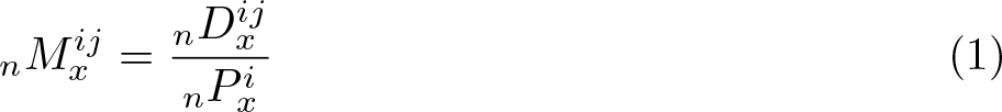
The input to calculate the functions of multistate life tables is a set of transition rates ² or survivorship proportions for age-specific groups. Formally, transition rates from state i to j between exact ages x and x + n are expressed as

${}_{n}M_x^{ij}=\frac{{}_{n}D_x^{ij}}{{}_{n}P_x^{ij}}$

1

where x, the lower right subscript, refers to the exact age at the beginning of each age interval and n, the lower left subscript, is the length of each age group, usually equal to one or five years in the demographic literature. To present and operationalize the data, one divides the continuous variable age—including decimal or fractional years—into a discrete set of categorical groups starting at exact times or ages x and ending after n years, the elapsed time in each interval. ${}_{n}D_x^{ij}$ is the observed number of transfers between states i and j, from exact age x to the instant before attaining exact age x + n. ³ ${}_{n}P_x^i$ comprises the midperiod population in state i between these same ages. So ${}_{1}M_{20}^{ij}$ , the transition rate from state i to j between ages 20 and 21, refers to events occurring to persons who are aged 20.0000 to 20.9999 in exact years since birth; and ${}_{5}M_{20}^{ij}$ would include the events and the population of individuals who have completed 20, 21, 22, 23, and 24 years of age since birth. Although the length of n depends on the type of data available to the analyst, mslt provides most precise results with single-year data (n = 1). If such data are not available, the recommendation is to smooth the multiyear data using splines, interpolation, or any other indirect method before entering the data into Stata.

Survivorship proportions, on the other hand, are defined as

${}_{n}S_x^{ij}=\frac{{}_{n}P_{x+n}^{ij}(t+n)}{{}_{n}P_x^{ij}(t)}$

2

where ${}_{n}P_x^i(t)$ is the number of persons in state i of the observed population between the ages of x and x + n at time t, and ${}_{n}P_{x+n}^{ij}(t+n)$ is the number of persons in state j of the observed population between the ages of x + n and x + 2n at time t + n who were in state i exactly n years earlier (Schoen 1988a). The key difference between (2) and (1) is that survivorship proportions rely on the same group of individuals, while rates may not.

Four methods—linear, mean duration at transfer, exponential, and cubic ⁴ —solve for the quantities of multistate life tables when transition rates are available. Alternatively, when data are entered as survivorship proportions and must be converted to rates, only two strategies—linear or exponential—are available (Schoen 1988a). mslt handles data of both types (rates and proportions) to provide linear and exponential solutions for multistate life tables. The other two alternatives (mean duration at transfer and cubic solutions) have not yet been incorporated into the program. Research has shown, however, that these methods “produce very similar values for single-year age intervals” (Schoen 1975, 1988a).

3 The mslt algorithms

This section presents formulas to estimate the functions and key summary measures of multistate life tables. Because of its technical content, readers not familiar with demographic notations may find it challenging to follow and may skip to the next section for an intuitive illustration of the method and straightforward interpretations of results. However, those who want to have a keen grasp of what mslt is assuming and doing are encouraged to read this section and to look further into its references.

The essential quantities of multistate life tables are the number of individuals in state i at exact ages x and x + n, $l_x^i$ , and $l_{x+n}^i$ . Under the assumption that $l_x^i$ is linear (increasing risk of the event within each age interval), the number of individuals at age x + n, $l_{x+n}^i$ , is calculated by solving the matrix equation originally suggested by Schoen (1975) and Rogers and Ledent (1976) and later referenced by Schoen (1988a, 70) and Palloni (2001, 269),

$\text{l}(x+n)=\text{l}(x)\left\{\text{I}-\frac{n}{2}\text{M}(x,n)\right\}{\left\{\text{I}+\frac{n}{2}\text{M}(x,n)\right\}}^{-1}$

3

where l(x + n) and l(x) are row vectors containing the numbers of individuals in states of interest, I is the identity matrix, n represents, as in (1) and (2), the length of age intervals, M(x, n) are square matrices containing transition rates from state i and j and between exact ages x and x + n, and the superscript −1 indicates the matrix inverse. Each age group—defined by and between ages x and x + n—has a set of age-specific transition rates. Each age group between the first and the last age x has its own matrix M(x, n). The integer values assumed by x and n (usually 1 or 5) may vary according to the analyst’s dataset and are thus left unconstrained.

In particular, in the presence of an absorbing state, ⁵ the structure of the (k + 1) by (k + 1) matrix of observed transition rates from state i to state j between ages x and x + n is

$\text{M}(x,n)=\begin{array}{ccccc}{\displaystyle \sum {\hspace{0.17em}}_n{M}_x^{1,j}}& {-}_n{M}_x^{1,2}& \cdots & {-}_n{M}_x^{1,k}& {-}_n{M}_x^{1,k+1}\\ {-}_n{M}_x^{2,1}& {\displaystyle \sum {\hspace{0.17em}}_n{M}_x^{2,j}}& \cdots & {-}_n{M}_x^{2,k}& {-}_n{M}_x^{2,k+1}\\ ⋮& ⋮& \ddots & ⋮& ⋮\\ {-}_n{M}_x^{k,1}& {-}_n{M}_x^{k,2}& \cdots & {\displaystyle \sum {\hspace{0.17em}}_n{M}_x^{k,j}}& {-}_n{M}_x^{k,k+1}\\ 0& 0& \hspace{0.17em}& 0& 0\end{array}$

4

where the summations over j run from 1 to k + 1 possible destinations for a person in one of the k living states, excluding the case where j = i.

Notice that each row in (4) sums to 0 and that the diagonal elements are a sum of the transition rates in the same row. In the absence of an absorbing state, the elements of the last row and column of matrix M(x, n) should be excluded. Alternatively, according to Rogers and Ledent (1976) and Ledent and Zeng (2010), matrix M(x, n) could be transposed and have death rates included in the main diagonal instead of in the last row and column.

Alternatively, under the assumption that rates are constant in age intervals, the solution, first used by DuPasquier (1912) and later applied by Krishnamoorthy (1979) to investigate marital statuses, can be expressed as

$l(x+n)=l(x)\hspace{0.17em}\text{exp}\{-nM(x,n)\}$

5

where

$\text{exp}\{-nM(x,n)\}+\text{I}-n\text{M}(x,n)+\frac{n^2}{2!}{\text{M}}^2(x,n)-\frac{n^3}{3!}{\text{M}}^3(x,n)\dots$

6

If the rates in M(x, n) are small, the values on the left of (6) will usually stabilize after the second or third element in the infinite power series. ⁶

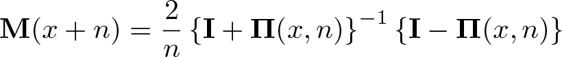
If instead of rates one enters survivorship proportions ${\hspace{0.17em}}_n{S}_x^{ij}$ , the option proportion, in the mslt command, must be requested to convert such values to rates before calculating the remaining functions of the multistate table. Under the linear assumption, following Schoen (1988a) and Rees and Wilson (1977), this conversion is done by solving two matricial equations,

$\text{M}(x+n)=\frac{2}{n}{\{\text{I}+\text{II}(x,n)\}}^{-1}\{\text{I}-\text{II}(x,n)\}$

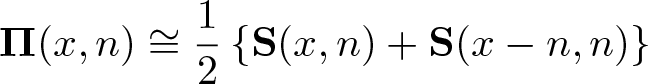
in which

$\text{II}(x+n)\cong \frac{1}{2}\{\text{S}(x,n)+\{S(x-n,n)\}$

where S(x, n) has element ${\hspace{0.17em}}_n{S}_x^{ij}$ in the ith row and jth column, with restricted values between 0 and 1. The structure of square matrix Π(x, n) is not the same as M(x, n), so mslt invokes different Mata functions when the option proportion is inserted in the command line. In particular, in the presence of an absorbing state, the (k+1) by (k+1) square matrix of observed transition probabilities is

$\prod (x,n)=\begin{array}{cccc}{\hspace{0.17em}}_n{\pi }_x^{11}& {\hspace{0.17em}}_n{\pi }_x^{12}& \cdots & {\pi }^{1,k+1}\\ {\hspace{0.17em}}_n{\pi }_x^{21}& {\hspace{0.17em}}_n{\pi }_x^{22}& \cdots & {\pi }^{2,k+1}\\ ⋮& ⋮& \ddots & ⋮\\ 0& 0& \hspace{0.17em}& 1\end{array}$

7

Each row in (7) sums to 1, and in the absence of an absorbing state, the elements in the last row and column should be excluded. As an alternative compact form, if one added the probabilities of moving to the absorbing state to the main diagonal, matrix Π(x, n) could have as its elements interstate transition probabilities arranged in transposed order (Rogers and Ledent 1976).

Under the constant risks assumption, the conversion of probabilities to rates is approximate by the matrix logarithm solution offered by Hall (2015):

$\begin{array}{c}\text{M}(x,n)=-\frac{1}{n}{\displaystyle \sum _{k=1}^{\infty }{(-1)}^{k=1}\frac{{\{\text{Π}(x,n)-\text{I}\}}^k}{k}}\\ =-\frac{1}{n}\left[\{\text{Π}(x,n)-\text{I}\}-\frac{{\{\text{Π}(x,n)-\text{I}\}}^2}{2}+\frac{{\{\text{Π}(x,n)-\text{I}\}}^3}{3}\cdots \right]\end{array}$

Once matrices M(x, n) and vectors l(x) are obtained through linear or exponential solutions, the other functions of the multistate life table are straightforward. Continuing with matrix notation, under the linear assumption and following (3), we give the number of transitions from state i to j between ages x and x + n by the off-diagonal elements of

$\begin{array}{c}{\text{D}}_1(x,n)=\text{diag}\{\text{l}(x)\}\left\{\text{I}-\frac{n}{2}\text{M}(x,n)\right\}{\left\{\text{I}+\frac{n}{2}\text{M}(x,n)\right\}}^{-1}\\ =\left(\begin{array}{cccc}{l}_{x+n}^{11}& {\hspace{0.17em}}_n{d}_x^{12}& \cdots & {\hspace{0.17em}}_n{d}_x^{1,k+1}\\ {\hspace{0.17em}}_n{d}_x^{21}& l_{x+n}^{22}& \cdots & {\hspace{0.17em}}_n{d}_x^{2,k+1}\\ ⋮& ⋮& \ddots & ⋮\\ 0& 0& \hspace{0.17em}& l_{x+n}^{k+1,k+1}\end{array}\right)\end{array}$

8

where the diagonal elements $l_{x+n}^{ii}$ represent the number of individuals in the cohort who are in state i at age x+n after accounting for the outflows from state i to j presented in the same row (but without considering the inflows from j to i). ⁷ Under the constant forces assumption, following a slight variation of (5), the analogous matrix of D _l(x, n) is

$D_{\text{c}}(x,n)=\text{diag}\{l(x)\}\hspace{0.17em}\text{exp}\hspace{0.17em}\{-nM(x,n)\}$

9

which, in longhand form, has elements structured in the same way as in D _l(x, n). However, the value of the elements in D _c(x, n) differ to reflect the assumption of constant risks of the event within age intervals.

In the absence of an absorbing state, matrices D _l(x, n) and D _c(x, n) do not have their last rows and columns. After executing (8) or (9) for all ages, mslt removes the main diagonal and columns with zero decrements (that is, in which i = j or in which i is an absorbing state) and provides a rearranged array d(x, n) for the number of transitions from state i to state j between ages x and x + n. This matrix is saved in Mata as

$\text{d}(x,n)=\left(\begin{array}{ccc}{\hspace{0.17em}}_n{d}_x^{ij}& \cdots & {\hspace{0.17em}}_n{d}_x^{k,k+1}\\ {\hspace{0.17em}}_n{d}_{x+n}^{ij}& \cdots & {\hspace{0.17em}}_n{d}_{x+n}^{k,k+1}\\ {\hspace{0.17em}}_n{d}_{x+2n}^{ij}& \cdots & {\hspace{0.17em}}_n{d}_{x+2n}^{k,k+1}\\ ⋮& \hspace{0.17em}& ⋮\\ {\hspace{0.17em}}_n{d}_{x+\lambda n}^{ij}& \cdots & {\hspace{0.17em}}_n{d}_{x+\lambda n}^{k,k+1}\end{array}\right)$

where λ represents the number of age groups in the dataset and, as before, k accounts for the number of nonabsorbing states and k + 1 destinations (including death). Columns of d(x, n) are indexed by states of origin i and destination j; rows identify age intervals of length n; the first age interval starts at age x and the last at age x + λn.

The probabilities that an individual in state i at exact ages x will occupy state j at ages x + n can then be obtained as

${\hspace{0.17em}}_n{q}_x^{ij}=\frac{{\hspace{0.17em}}_n{d}_x^{ij}}{l_x^i}$

Under the linear assumption, the number of person-years lived in state i between exact ages x and x + n can be approximated by the arithmetic mean of the number of survivors times the length of the age interval:

$\text{L}(x,n)=\frac{n}{2}\{\text{l}(x)+\text{l}(x+n)\}$

10

And under the exponential assumption, we obtain the number of person-years by solving the expression ⁸

$\text{L}(x,n)=n\text{l}(x)\left\{\frac{n}{2!}\text{M}(x,n)+\frac{n^2}{3!}{\text{M}}^2(x,n)-\frac{n^3}{4!}{\text{M}}^3(x,n)\cdots \right\}$

In the presence of an absorbing state and a last open-ended age group (that is, not constrained by a length of n, as in the case of all other age groups), the vector of person-years in the last time interval is ⁹

$\text{L}(x,\infty )=\text{l}(x,\infty )\left(\begin{array}{cccc}{\hspace{0.17em}}_{\infty }{M}_x^{1d}+{\displaystyle \sum {\hspace{0.17em}}_{\infty }{M}_x^{1j}}& {-}_{\infty }{M}_x^{21}& \cdots & {-}_{\infty }{M}_x^{k1}\\ {-}_{\infty }{M}_x^{12}& {\hspace{0.17em}}_{\infty }{M}_x^{2d}+{\displaystyle \sum {\hspace{0.17em}}_{\infty }{M}_x^{2j}}& \cdots & {-}_{\infty }{M}_x^{k2}\\ ⋮& ⋮& \ddots & ⋮\\ {-}_{\infty }{M}_x^{1k}& {-}_{\infty }{M}_x^{2k}& \hspace{0.17em}& {\hspace{0.17em}}_{\infty }{M}_x^{kd}+{\displaystyle \sum {\hspace{0.17em}}_{\infty }{M}_x^{kj}}\end{array}\right)$

11

where each diagonal element contains the total rate of exit of state k—rates of mortality ${\hspace{0.17em}}_{\infty }{M}_x^{kd}$ plus mobilities ${\displaystyle \sum {\hspace{0.17em}}_{\infty }{M}_x^{kj}}$ to state j—while the off-diagonal elements represent rates of moving from state j to k preceded by a minus sign. ¹⁰

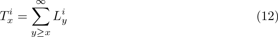
After we use Baum’s (2006) neat function to put matrices upside down, the number of person-years lived in state i above age x is

$T_x^i={\displaystyle \sum _{y\ge x}^{\infty }{L}_y^i}$

12

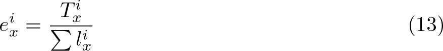
Unconditional (or population-based) life expectancy at age x in state i is

$e_x^i=\frac{T_x^i}{{\displaystyle \sum l_x^i}}$

13

Notice that the denominator in (13) includes all survivors at age x, regardless of state of occupancy at that same age (Guillot 2015). The unconditional life expectancy refers to the number of years to be lived in state i after age x. It is “the average number of person-years lived in state i at and above exact age $x\hspace{0.17em}[T_x^i]$ by all persons alive at exact age $x\hspace{0.17em}[{\displaystyle \sum l_x^i}]$ ” (Schoen 1988a, 83).

Alternatively, to calculate conditional (or status-based) life expectancies at age x in state j, for individuals who are in state i at age x, we use

$e_x^{ij}=\frac{T_x^{ij}}{l_x^i}$

14

The conditional life expectancy “reflects the average number of future years lived in state $j\hspace{0.17em}[T_x^{ij}]$ by the closed group of persons in state i at exact age $x\hspace{0.17em}[l_x^i]$ ” (Schoen 1988a, 84). Conditional life expectancies refer to the lived experience of a single cohort born at a given age and in just one state $(l_x^i,T_x^{ij})$ , while unconditional life expectancies combine the experience of cohorts born in all states $\left({\displaystyle \sum l_x^i,T_x^i}\right)$ . ¹¹

In addition, when summary is invoked, and depending on whether death is also specified, mslt produces the following summary measures (SM) (Schoen 1988a, 95):

Proportion of life spent in state i:

${\text{SM}}_1^i=\frac{T_0^i}{{\displaystyle \sum T_0^i}}$

15

Probability of dying in state i,

${\text{SM}}_2^i=\frac{{\displaystyle \sum {\hspace{0.17em}}_n{d}_x^{i\delta }}}{{\displaystyle \sum l_0^i}}$

where δ represents the absorbing state.

Average duration of state i:

${\text{SM}}_3^i=\frac{T_0^i}{{\displaystyle \sum {\hspace{0.17em}}_n{d}_x^{ji}}}$

16

Mean age at transfer from state i to j:

${\text{SM}}_4^i=\frac{{\displaystyle \sum (x+\frac{n}{2})d_x^{ij}}}{{\displaystyle \sum {\hspace{0.17em}}_n{d}_x^{ij}}}$

Mean age of persons in state i:

${\text{SM}}_5^i=\frac{{\displaystyle \sum (x+\frac{n}{2})L_x^i}}{T_0^i}$

17

For convenience, these quantities are saved in Mata and, for the sake of presentation, also as Stata matrices. When the inputs of mslt—occurrence rates or proportion of survivors—are not available, one can still obtain them by aggregating individual estimates, produced by event history (Cleves, Gould, and Marchenko 2016) or probability models (Long and Freese 2014), into population-level rates by age. The advantage of these microlevel approaches is that they are able to incorporate individual heterogeneities into the transitions; that is, individuals in state i at age x must not assume the same probability of experiencing a transition (Guillot 2015).

4 Extended examples

To illustrate and validate the results of mslt, I use information describing children’s experience of cohabitation, marriage, or union disruption (Palloni 2001). The original data source is the National Survey of Family Growth, conducted in 1995 with 10,847 women between 15 and 44 years of age (Bumpass and Lu 2000). The survey contains retrospective information on union and fertility histories during the previous five years, which allows the calculation of transition rates between marital statuses. Figure 1 portrays, diagrammatically, the state-space of marital transitions.

Figure 1.

Multistate-space representation of children’s transitions between their mothers’ marital experience

In this representation, the stages of union formation and disruption are sequentially numbered, and the transition rates between them are indexed, so that the first superscript corresponds to the state of origin and the second to the state of destination. For example, ${\hspace{0.17em}}_n{M}_x^{13}$ represents the rate at which children who live with mothers who are not in a union experience a change between exact ages x and x + n and begin to live with a married female parent. Transitions to the absorbing state (Death) are in boldface, and widowhood, separation, and divorce states are not considered in this application. In the following section, I demonstrate the use of mslt in the absence of an absorbing state. Afterward, I simulate a situation in which death is included.

4.1 No absorbing state

This first example neglects the presence of death as an absorbing state. In such situation, the appropriate structure for a dataset containing transition rates ¹² of children 0 to 14 years old according to their mother’s marital status (1 = nonunion, 2 = cohabitation, 3 = marriage) is from the National Survey of Family Growth, apud Palloni (2001, 262). ¹³ The suffixes in the variable names represent, respectively, the marital states of origin i and destination j: 1 is for mothers not in unions; 2 indicates cohabitation; and 3 indexes marriage.

The first column must always define the lower limit of exposure time (usually age) in a given age group. The remaining columns are observed transition rates from state i to state j in age group x to x + 1, ₁ Mx^ij . For example, the rate of a child aged 0 who lived with a mother not in a union to live with a cohabiting mom is, by age 1, 0.0777. Also notice that the rates of permanence in the same state (that is, m11, m22, and m33) are purposefully omitted and should not be part of the working data.

Once a dataset with this structure and variables is entered into Stata, we are ready to explore the full potential of mslt. ¹⁴

Unconditional (population-based) life expectancies

To estimate the unconditional duration of time lived in a particular state (13) by all individuals who were in a given age x, mslt requires the number of births in each state i, l0 ⁱ . For example, by setting a radix of l0 ⁱ = 1000 for every i state (even though it likely varies according to the number of registered births in each condition) and after assuming that transition rates are constant within age intervals, we obtain multistate life-table functions (option matrix) and key summary measures by typing

In this particular example, because the last age group is not open ended (ending in x+n instead of x+∞), the option censored must be specified to avoid the assumption that everybody must die in the last age group (see footnote 9).

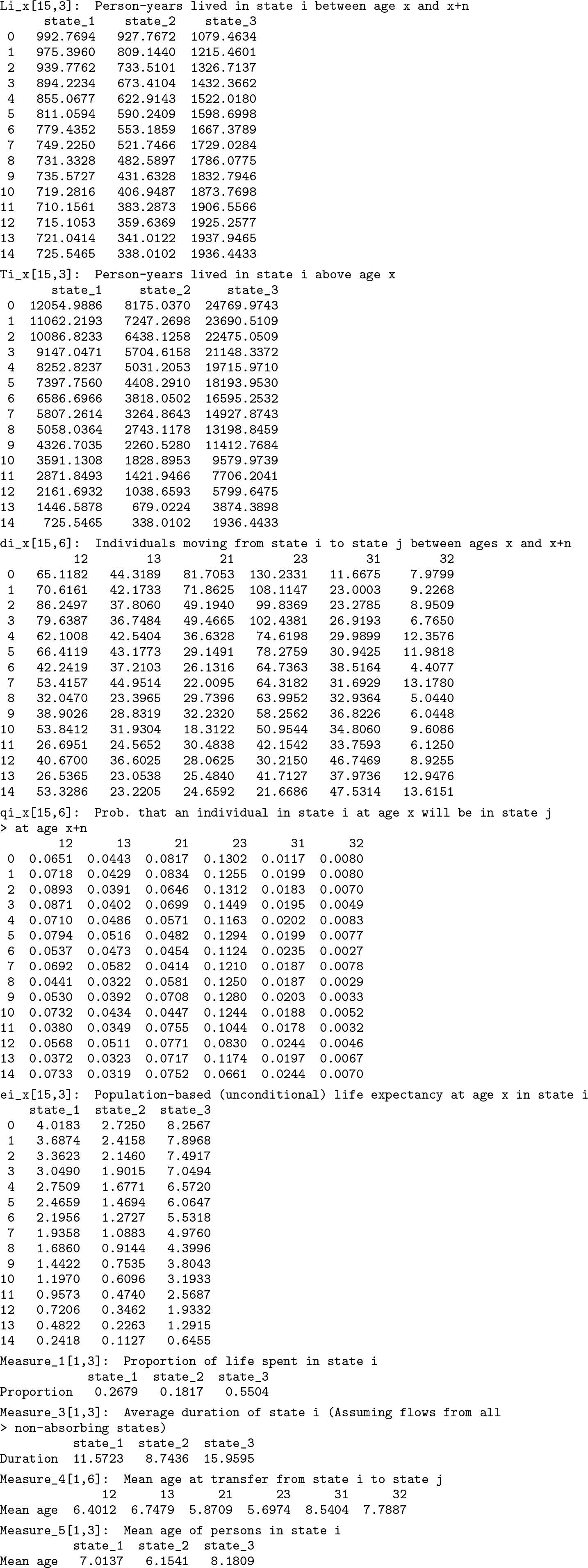
Quantities $(l_x^i{,}_n{d}_x^{ij}{,}_n{q}_x^{ij},e_x^i)$ are analogous to those reported by Palloni (2001); hence, they have the same interpretation. Matrix li_x shows the number of individuals at each exact age and state. The quantities can increase or decrease, depending on the flows ${\hspace{0.17em}}_n{d}_x^{ij}$ from states i to j in specific age groups.

Matrices di_x and qi_x show exits and transition probabilities between all nonabsorbing states. ¹⁵ According to matrix di_x, for example, between ages 0 and 1, ${\hspace{0.17em}}_1{d}_0^{12}=65$ individuals left state 1 (nonunion) for state 2 (cohabitation), and ${\hspace{0.17em}}_1{d}_0^{13}=44$ left state 1 for state 3 (marriage). During the same period of one year, ${\hspace{0.17em}}_1{d}_0^{21}=82$ individuals moved from state 2 to 1, and ${\hspace{0.17em}}_1{d}_0^{31}=12$ moved from state 3 to 1. As a result of these 109 exits and 93 entrances, there were 984 children living in state 1 at exact age 1, $l_1^1$ . Note that $l_1^1+l_1^2+l_1^3=l_1=3000$ , the total number of cohort members at age x = 1. In this example, because there is no mortality or any other absorbing state, this number equals to the sum of birth cohorts at all ages.

Another matrix of interest is qi_x, which shows six transition probabilities between three different states. The first column, ${\hspace{0.17em}}_1{q}_x^{12}$ , shows the probability for children who lived with a mother not in a union (state 1) at age x to live with a cohabiting mother (state 2) at age x + 1. At age 10, for example, a child in state 1 has three possibilities: a) to live with a cohabiting mother, with probability ${\hspace{0.17em}}_1{q}_{10}^{12}=7.32\%$ ; b) to live with a married mother, ${\hspace{0.17em}}_1{q}_{10}^{13}=4.34\%$ ; or to remain in the current living arrangement with a mother not in a union, ${\hspace{0.17em}}_1{q}_{10}^{11}=88.34\%$ . Needless to say, these three probabilities add up to 100%, and a similar interpretation applies to the other columns or states. ¹⁶

Matrix ei_x, which summarizes the mean duration of state occupancy above age x, shows that in the first 15 years of their lives, children could expect to experience 4.02 years in state_1 (nonunion), 2.73 years in state_2 (cohabitation), and 8.26 years in state_3 (married). They will spend, therefore, most of the initial stages of their lives living in a family with married mothers. For ease of visualization, life expectancies are automatically plotted in a graph (see figure 2), which could be further edited and optionally saved by the user.

Figure 2.

Unconditional life expectancies by age

The other two matrices, Li_x and Ti_x, account for person-years lived in state i. ${\hspace{0.17em}}_1{L}_0^1=992.77$ , for example, represents the number of person-years at risk of experiencing a transition from state 1 to state j between exact ages 0 and 1. And $T_0^1=12,054.99$ corresponds to the cumulative sum of ${\hspace{0.17em}}_1{L}_{14}^1$ to ${\hspace{0.17em}}_1{L}_0^1$ , as generally stated in (12). The meanings of ${\hspace{0.17em}}_n{L}_x^i$ and $T_x^i$ , per se, are not intuitive for nondemographers unfamiliar with the concept of person-years. They are, however, fundamental steps to calculate important quantities of multistate life tables, shown in (13), (14), (15), (16), (17).

Finally, an added virtue of mslt is to produce key measures of interest, which show that about half (55.04%) of children’s first 15 years will be spent with married mothers; that cohabitations have an average total (and not necessarily consecutive) duration of 8.7 years; that children move from the nonunion to the married state when they are about 6.75 years old; and that those living with married mothers are, on average, 8.18 years old.

Conditional (status-based) life expectancies

Conditional life expectancies are the predicted number of years to be lived in state j by those who are in state i at exact age x [see (14)]. They differ from unconditional estimates by considering the lived experience of a single cohort, born in just one (conditional) state. The strategy to obtain the quantities $T_x^{ij}$ , required to estimate conditional life expectancies, is to recalculate the model with all persons born just in the (conditional) state and age of interest. By setting the number of “births” in the other cohorts and states to zero and requesting the option conditional, we specify that mslt produce status-based life expectancies at every age. For instance, by recalling mslt with 1,000 “births” at every age only in the nonunion state, we obtain the number of expected years lived in every state by those who were in state_1 at exact age x:

Conditional life expectancy at birth (7.86 years)—for children who were born and were living with mothers out of wedlock—is about twice larger than previously estimated unconditional life expectancy (4.02 years) in state_1 at that same age—for children born in any state. Therefore, the average number of future years lived in state_1 by a closed group of persons in state_1 at age x is almost two times larger than the number of years lived regardless of the state of origin. If we had instead set l0(0 1000 0) or l0(0 0 1000), we would have obtained, respectively, conditional life expectancies for states 2 and 3.

To calculate conditional life expectancies, mslt generates a set of $l_x^i,L_x^{ij}$ , and $T_x^{ij}$ matrices for each age group and nonabsorbing state. Thus, in this particular example, 45 sets are generated (one for each of the 15 age groups in each of the 3 states). For instance, conditional life expectancies at ages 4 and 5 were respectively calculated from state-specific rows in Mata matrices ( $T_4^{1j}=\text{T}5[5,.],\hspace{0.17em}{l}_4^1=\text{l}5[5,1]=1000$ ; and $T_5^{1j}=\text{T}6[6,.],\hspace{0.17em}{l}_5^1=\text{l}6[6,1]=1000$ ):

In this example, the starting radix ( $l_x^1=1000$ ) is entered 15 times in state 1, once for each age group, to obtain the appropriate values of $T_x^{ij}$ for every starting age of interest. Only the initial radix (that is, 1,000) was used in the denominator of (14). Life expectancies conditional on those who were in state 2 (that is, mslt, l0(0 1000 0) conditional) would use the same initial value in the denominator of (14), but the number of person-years lived in state j above age x, the numerator $T_x^{ij}$ , would change accordingly.

The options matrix and summary are not available when conditional is specified because it generates several (135 in this case) state-specific Mata matrices to derive status-based life expectancies at ages x and not only one set, as in the case of populationbased (unconditional) life expectancies.

4.2 Incorporating an absorbing state (exempli gratia, death)

mslt is capable of handling any number of nonabsorbing states and, at most, one absorbing state. We now turn, therefore, to an example with four states, in which “4.death” is a possibility. Variables m12, m13, m21, m23, m31, and m32 are the same as in section 4.1, but the data now also include transitions from nonunion, cohabitation and marriage statuses to death (that is, m14, m24, and m34). Note that the data from the National Survey of Family Growth now include randomly generated death rates. Also note that the suffixes in the variable names represent, respectively, the marital states of origin i and destination j: 1 is for mothers not in unions; 2 indicates cohabitation; 3 indexes marriage; and 4 represents the death state.

The mortality rate for a child aged 0, who lived with a mother not in a union (m14), is 0.008. Notice that a) transitions to the absorbing state (m14, m24, m34) should be the last column within each nonabsorbing state of analysis; b) there are, by definition, no decrements from the absorbing state (that is, no m41, m42, and m43 variables); and c) the last age group is censored, instead of open ended. With an absorbing state, the option death must be declared, and the last value in l0( numlist ) must be zero. Once again, assuming constant force of mortality, unconditional life expectancies and summary measures are obtained by entering the following command line:

Unconditional life expectancies at birth for state_1, state_2, and state_3 are now 3.46, 2.15, and 7.20 years. And conditional values could be obtained as before, by recalling mslt with the option conditional and zeros in specific states of l0( numlist ).

Measure_1 shows that individuals, respectively, spend 23%, 14%, and 48% of their lives in states 1, 2, and 3 (the remaining 15% accounts for those who died). When there is an absorbing state and the option summary is requested, mslt reports the probability of dying in state i, Measure_2. In our example, it shows that the probability of dying in state_1 is 7.43% and in state_2 is 11.48%.

Multistate life-table functions are saved as Mata and as Stata matrices and can be listed accordingly. To list ₁ dx^ij , the number of transitions from state i to state j between exact ages x and x + 1, for example, one could invoke

One of the values in matrix di_x shows, for example, that from exact ages 10 to 11, 57 children moved from states 1 to 4, ${\hspace{0.17em}}_1{d}_{10}^{14}=56.713$ deaths. This number is about eight times higher than the quantity of children who made transitions from state 3 to state 2 at the same age interval, ${\hspace{0.17em}}_1{d}_{10}^{32}=7.626$ .

Mata and Stata commands report the same values, but if the option matrix had been called with mslt, a neat title for each multistate function would have been displayed. Graphs of Mata matrices can be produced with function mm_plot(), available in Jann’s (2005a) moremata, or by converting Stata matrices to variables using svmat (see [M-4] Matrix) for manipulation with twoway plots (see [G-2] graph).

5 The mslt command

5.1 Syntax

mslt, l0( numlist ) [proportion constant death censored conditional matrix summary]

5.2 Description

The most important quantities in increment–decrement tables are conditional and unconditional life expectancies, which summarize the average duration of time spent in a particular state i above a given age x. mslt calculates the functions ( $l_x^i,{\hspace{0.17em}}_n{L}_x^i,\hspace{0.17em}{T}_x^i,{\hspace{0.17em}}_n{d}_x^{ij},{\hspace{0.17em}}_n{q}_x^{ij},\hspace{0.17em}{e}_x^i,\hspace{0.17em}{e}_x^{ij}$ ) of increment–decrement life tables following the methods and procedures described in Rogers and Ledent (1976), Schoen (1988a), and Palloni (2001). By specifying the summary option, mslt also calculates mean ages, proportions of life, and probabilities of dying in a given state. The inputs for mslt are

transition rates (or survivorship proportions) between various states by age; and

the initial number of individuals in each cohort and state.

An adequate dataset, before entered into Stata, should have the same structure and order of variables described in the examples of sections 4.1 and 4.2.

By default, mslt assumes that rates are the working input and that the underlying risks of transition are linear within age intervals. Users can, however, optionally enter survivorship proportions (that is, proportion) and assume constant rates in each age interval. Doing so will calculate the number of survivors in the cohort in state i and age x, function $l_x^i$ , using the exponential method.

5.3 Options

l0( numlist) lists the initial number of individuals in each cohort and state. Traditionally, these radices are set as multiples of hundreds (1,000, 10,000, etc.), but the user is allowed to enter other values. A suitable option is to consider the actual distribution of births by state, as observed in the populations under investigation. In a situation with three nonabsorbing and one absorbing state, four values must be provided, and the last one of them is necessarily zero because people cannot be born in an absorbing state. The numlist in such a situation could be, for example, l0(1000 1000 1000 0). l0() is required.

proportion declares that the input data refer to survivorship proportions instead of rates. When one enters this option, mslt converts proportions to probabilities and then to rates under the linear assumption. If the option constant is simultaneously informed, the conversion is made under the constant forces assumption.

constant implements the exponential solution, under the constant forces assumption, to calculate the number of individuals in state i at exact age x, $l_x^i$ . It should be declared whenever this function is nonlinear (exponential) with age or the underlying risks are relatively stable. Otherwise, “the exponential method produces somewhat inaccurate values in cases where the transition probabilities are increasing or decreasing rapidly” (Schoen 1988a, 75–76).

death declares the presence of an absorbing state. This option should be included whenever there is a state to which people are able to enter but not leave. Examples of absorbing states are death, schooling, and incurable diseases.

censored declares that the last age interval is censored (that is, ending in x+n), instead of open ended (ending in x + ∞). To warrant an accurate calculation of the number of person-years, one must specify this option whenever the last age group is not open ended.

conditional calculates life expectancies conditional on state of occupancy at age x and must be properly combined with births in just one state in l0( numlist ). By default, mslt estimates unconditional life expectancies.

matrix tells mslt to display matrices on the screen containing the key functions ( $l_x^i,\hspace{0.17em}{L}_x^i,\hspace{0.17em}{T}_x^i,{\hspace{0.17em}}_n{d}_x^{ij},{\hspace{0.17em}}_n{q}_x^{ij},\hspace{0.17em}{e}_x^i$ ) of increment–decrement life tables for each state i and at exact ages x. This option cannot be specified with the option conditional.

summary displays summary measures for multistate life tables. It reports the proportion of life spent in state i (Measure_1), the average age of persons in state i (Measure_5), the average duration of state i (Measure_3)—assuming the presence of flows between all nonabsorbing states—and the mean age at transfer from state i to state j (Measure_4). Finally, if death is simultaneously requested, summary shows the probability of dying in state i (Measure_2). This option is not available when status-based life expectancies (that is, conditional) are requested.

5.4 Output

As a minimum, mslt displays a table and a graph of life expectancies by state and time. With option matrix, it shows matrices of multistate functions on the screen, and with option summary, it displays summary measures of multistate life tables.

5.5 Stored results

Multistate life-table functions are stored in Mata (without the “i_ x” suffix) and as Stata matrices under the following names:

Supplemental Material

Supplemental Material, st0615 - Multistate life tables using Stata

Supplemental Material, st0615 for Multistate life tables using Stata by Jerônimo Oliveira Muniz in The Stata Journal

References

1.
AlmG.1959. Connection between maturity, size, and age in fishes. Technical report, Drottningholm Institution Freshwater Research.
BumpassL.LuH.-H.2000. Trends in cohabitation and implications for children’s family contexts in the United States. Population Studies54: 29–41. https://doi.org/10.1080/713779060.
4.
CaswellH.2001. Matrix Population Models: Construction, Analysis, and Interpretation. 2nd ed. Sunderland, MA: Sinauer Associates.
5.
ClevesM.GouldW. W.MarchenkoY. V.2016. An Introduction to Survival Analysis Using Stata. Rev. 3rd ed. College Station, TX: Stata Press.
6.
DuPasquierL. G.1912. Mathematische theorie der invalidit¨atsversicherung. Mittleilungen der Vereinigung Schweizerischer Versicherungsmathematiker7: 1–17.
7.
GuillotM.2015. Multistate Transition Models in Demography. In International Encyclopedia of the Social and Behavioral Sciences, ed. WrightJ. D., 2nd ed., 109–115. Amsterdam: Elsevier. https://doi.org/10.1016/B978-0-08-097086-8.31019-4.
8.
HallB. C.2015. Lie Groups, Lie Algebras, and Representations: An Elementary Introduction. 2nd ed. Switzerland: Springer.
9.
HughesT. P.JacksonJ. B. C.1985. Population dynamics and life histories of foliaceous corals. Ecological Monographs55: 141–166. https://doi.org/10.2307/1942555.
10.
JacksonJ. B. C.1985. Distribution and ecology of clonal and aclonal benthic invertebrates. In Population Biology and Evolution of Clonal Organisms, ed. JacksonJ. B. C.BussL. W.CookR. E., 297–356. New Haven, London: Yale University Press. https://doi.org/10.2307/j.ctt2250w9n.12.
11.
JannB.2005a. moremata: Stata module (Mata) to provide various functions. Statistical Software Components S455001, Department of Economics, Boston College. https://ideas.repec.org/c/boc/bocode/s455001.html.
JiménezJ. A.LugoA. E.CintrónG. . 1985. Tree mortality and mangrove forests. Biotropica17: 177–185.
15.
KrishnamoorthyS.1979. Classical approach to increment-decrement life tables: An application to the study of the marital status of United States females, 1970. Mathemathical Biosciences44: 139–154. https://doi.org/10.1016/0025-5564(79)90033-6.
16.
LandK. C.GuralnikJ. M.BlazerD. G.1994. Estimating increment-decrement life tables with multiple covariates from panel data: The case of active life expectancy. Demography31: 297–319. https://doi.org/10.2307/2061887.
17.
LedentJ.1980. Multistate life tables: Movement versus transition perspectives. Environment and Planning A: Economy and Space12: 533–562. https://doi.org/10.1068/a120533.
18.
LedentJ.ZengY.2010. Multistate Demography. In Encyclopedia of Life Support Systems, vol. 2, ed. ZengY., 139–163. Oxford: EOLSS Publishers/Unesco.
19.
LefkovitchL. P.1965. The study of population growth in organisms grouped by stages. Biometrics21: 1–18. https://doi.org/10.2307/2528348.
20.
LongJ. S.FreeseJ.2014. Regression Models for Categorical Dependent Variables Using Stata. 3rd ed. College Station, TX: Stata Press.
21.
LutzW.GoujonA.2001. The world’s changing human capital stock: Multi-state population projections by educational attainment. Population and Development Review27: 323–339. https://doi.org/10.1111/j.1728-4457.2001.00323.x.
22.
PalloniA.2001. Increment-decrement life tables. In Demography: Measuring and Modeling Population Processes, ed. PrestonS. H.HeuvelineP.GuillotM., 256–272. Oxford: Blackwell.
23.
ReesP. H.WilsonA. G.1977. Spatial Population Analysis. London: Arnold.
SchoenR.LandK. C.1979. A general algorithm for estimating a Markovgenerated increment-decrement life table with applications to marital-status patterns. Journal of the American Statistical Association74: 761–776. https://doi.org/10.1080/01621459.1979.10481029.
31.
SmithS. J.1982. Tables of working life: The increment-decrement model, Bulletin 2135. Washington, DC: U.S. Dept. of Labor, Bureau of Labor Statistics. http://catalog.hathitrust.org/Record/011408963.
32.
SomertonD. A.MacIntoshR. A.1983. The size at sexual maturity of blue king crab, Paralithodes platypus, in Alaska. Fishery Bulletin81: 621–628.
33.
UsherM. B.1966. A matrix approach to the management of renewable resources, with special reference to selection forests. Journal of Applied Ecology3: 355–367. https://doi.org/10.2307/2401258.
WillekensF. J.1980. Multistate analysis: Tables of working life. Environment and Planning A: Economy and Space12: 563–588. https://doi.org/10.1068/a120563.
36.
YangY.WalijM.2010. Increment-decrement life table estimates of happy life expectancy for the U.S. population. Population Research and Policy Review29: 775–795. https://doi.org/10.1007/s11113-009-9162-5.
37.
ZonR.1915. Seed production of western white pine. Technical report, Bulletin No. 210, Department of Agriculture.
Supplementary Material
Please find the following supplemental material available below.
For Open Access articles published under a Creative Commons License, all supplemental material carries the same license as the article it is associated with.
For non-Open Access articles published, all supplemental material carries a non-exclusive license, and permission requests for re-use of supplemental material or any part of supplemental material shall be sent directly to the copyright owner as specified in the copyright notice associated with the article.