Uniform nonparametric inference for time series using Stata

Abstract

In this article, we introduce a command, tssreg, that conducts nonparametric series estimation and uniform inference for time-series data, including the case with independent data as a special case. This command can be used to nonparametrically estimate the conditional expectation function and the uniform confidence band at a user-specified confidence level, based on an econometric theory that accommodates general time-series dependence. The uniform inference tool can also be used to perform nonparametric specification tests for conditional moment restrictions commonly seen in dynamic equilibrium models.

1 Introduction

Nonparametric problems arise routinely from applied work because the economic intuition of the guiding economic theory often does not depend on stylized parametric model assumptions. A leading approach is to approximate the unknown function using a large number of basis functions; see, for example, Andrews (1991), Newey (1997), Chen (2007), Belloni et al. (2015), and Chen and Christensen (2015). The series estimation method is intuitively appealing, and an empirical researcher’s “flexible” regression specification can often be given a formal nonparametric interpretation as a series estimator.

In a companion article, Li and Liao (Forthcoming) propose an econometric method for making uniform nonparametric inference in a general time-series setting based on series estimation. The proposed uniform confidence band allows the empirical researcher to make a formal statistical statement on the entire conditional expectation function. This “global” inference differs from the conventional pointwise inference theory, as the latter only concerns the unknown function at a specific point and is thus “local” in nature. The inference method can also be conveniently used to conduct nonparametric specification tests for conditional moment restrictions that often stem from dynamic equilibrium models.

This article introduces the new command tssreg, which stands for time-series series regression. Based on the econometric theory in Li and Liao (Forthcoming), this command can be used to conduct two types of empirical analysis. One is to nonparametrically estimate a conditional expectation function and its uniform confidence band. The other is a sup-t test for conditional moment restrictions. We illustrate the method using the empirical example of Li and Liao (Forthcoming) and further extend their analysis.

This article is organized as follows. Section 2 provides some background on the underlying econometric method. Section 3 describes the basic features of the tssreg command. Section 4 provides a concrete illustration of the command in an empirical example and concludes.

2 Background on the uniform series inference method

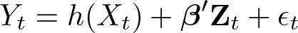
This section provides an overview of the econometric method. Consider the following nonparametric time-series regression,

$Y_t=h(X_t)+{\epsilon }_{t}E({\epsilon }_t|X_t)=0\text{1}\le t\le n$

where the dependent variable Y_t and the conditioning variable X_t are both univariate time series. Our econometric interest is to nonparametrically estimate the unknown function h(·) and make a uniform inference for it. More precisely, we aim to construct a (1 − α)-level confidence band $[\widehat{L}(·),\widehat{U}(·)]$ , such that

$P\left\{\widehat{L}(x)\le h(x)\le \widehat{U}(x)\text{ for all}\hspace{0.17em}x\in \chi \right\}\to \text{1}-\alpha$

1

as the sample size asymptotically goes to infinity, where χ is (possibly a subset of) the observed support of the conditioning variable.

We implement the econometric procedure proposed by Li and Liao (Forthcoming). These authors conduct nonparametric estimation using series regression and propose a confidence band that satisfies the uniform coverage property described in (1). Their method is justified by a strong approximation theory for time-series data. We refer the readers to Li and Liao (Forthcoming) for theoretical details.

The econometric procedure contains a few steps. In the first step, we conduct series estimation by regressing Y_t on a set of approximating functions of X_t , denoted by

$P(X_t)=\{p_{\text{1}}(X_t),...,p_m(X_t)\}\prime$

Among many possible choices of approximating functions, we use the following:

$p_j(x)=L_{j-}{\hspace{0.17em}}_{\text{1}}\{f(x)\}$

2

where L_j (·) denotes the jth Legendre polynomial, and f(·) is a fixed, strictly increasing transformation that serves the purpose of “rescaling” the conditioning variable X_t , as we will discuss in more detail below. The resulting regression coefficient is

$\widehat{\text{b}}={\left\{{\displaystyle \sum _{t=1}^n\text{P}\left(X_t\right)\text{P}(X_t{)}^{\prime }}\right\}}^{-1}\left\{{\displaystyle \sum _{t=1}^n\text{P}\left(X_t\right)Y_t}\right\}$

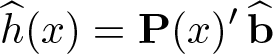
and the series estimator of h(x) is subsequently given by

$\widehat{h}(x)=P(x)\prime \widehat{b}$

The approximating functions in (2) are adopted to minimize the issue of multicollinearity, which is particularly relevant when the regression involves many series terms (that is, when m is large). To see how this works, let us first recall some basic properties of Legendre polynomials. These functions can be defined recursively as follows: L ₀(x) = 1, L ₁(x) = x, and

$L_j(x)=\frac{2j-1}{j}x{L}_{j-1}(x)-\frac{j-1}{j}{L}_{j-2}(x)j\ge 2$

Unlike the ordinary polynomial functions, the Legendre polynomials are orthogonal on the [−1, 1] interval with respect to the uniform distribution, that is, for j 6= k,

${\displaystyle {\int }_{-1}^1{L}_j(x)L_k(x)dx=0}$

If X_t is uniformly distributed over [−1, 1], the variables {L_j (X_t )} _{j≥ 0} are uncorrelated; hence, a regression on these variables does not suffer from the issue of multicollinearity. More generally, if the distribution function of X_t is F_X , the transformed variable f(X_t ), with f(x) = 2F_X (x)−1, is uniformly distributed over [−1, 1]. In this case, the regressors {p_j (X_t )}_1≤j≤m are mutually orthogonal. The tssreg command provides a few options for calibrating the f(·) transformation so as to “nearly” achieve this orthogonalization. By doing so, this command can accommodate a relatively large number of series terms without running into numerical instability issues. We also note that many other orthogonal basis functions, such as trigonometric series and Haar wavelets, may also be used for the same purpose. We do not intend to be exhaustive on these choices, leaving such extension to interested readers in the Stata community.

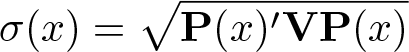
Li and Liao (Forthcoming) show that the estimation error $\widehat{h}(x)-h(x)$ can be approximately represented as P(x) ^′ξ in a well-defined theoretical sense, where ξ ∼ N(0, V) and V is the estimated variance–covariance matrix of $\widehat{b}$ . In the time-series context here, V generally accounts for serial dependence of the data, and we adopt the Newey–West estimator for this purpose (also see [TS] newey). The estimated standard error of $\widehat{h}(x)$ is thus

$\sigma (x)=\sqrt{P(x)\prime VP(x)}$

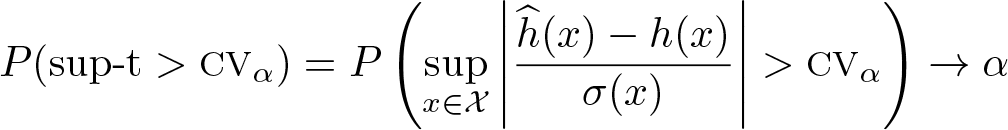
The uniform inference on the h(·) function is based on the sup-t statistic defined as

$\sup \text{-t}=\underset{x\in \chi }{\sup }|\frac{\widehat{h}(x)-h(x)}{\sigma (x)}|$

which can then be approximately represented by

$\underset{x\in \chi }{\sup }|\frac{\text{P}(x{)}^{\prime }\xi }{\sigma (x)}|$

Hence, we can compute the critical value (CV) at significance level α for the sup-t statistic, denoted by CV _α below, as the 1 − α quantile of this random variable. This computation is carried out via simulation, for which we draw ξ from the N(0, V) distribution and approximate χ with a subset of grid points for calculating the supremum.

It can be shown that in large samples

$P\left(\sup \text{-t}>{\text{cv}}_{\alpha }\right)=P\left(\underset{x\in \chi }{\sup }|\frac{\widehat{h}(x)-h(x)}{\sigma (x)}|>{\text{CV}}_{\alpha }\right)\to \alpha$

That is, the sup-t test provides correct size control under the null hypothesis

$H_0:E(Y_t|X_t=x)=h(x)\text{ all}\hspace{0.17em}x\in \chi$

We can also define the two-sided (1 − α)-level confidence band as

$\widehat{L}(x) = \widehat{h}(x) - {\text{CV}}_{\alpha }\sigma (x) \widehat{U}(x) = \widehat{h}(x) + {\text{CV}}_{\alpha }\sigma (x)$

which satisfies the desired uniform coverage property:

$P\left\{\widehat{L}(x)\le h(x)\le \widehat{U}(x)\text{ for all}\hspace{0.17em}x\in \chi \right\} \to \text{1}-\alpha$

The uniform confidence band is directly useful for making functional inference on the relation between the dependent variable Y_t and the conditioning variable X_t . Changing the perspective slightly, we further note that this method can be conveniently used to test conditional moment restrictions. Dynamic equilibrium models often imply conditional moment restrictions of the form

$E\{g(Y_t^{*};{\gamma }_0)|X_t\}=0$

where $Y_t^{*}$ is an observed time series and γ0 is a finite-dimensional vector of structural parameters. We can test this conditional moment restriction by nonparametrically regressing $Y_t=g(Y_t^{*};{\gamma }_0)$ on X_t . If the parameter γ0 is unknown, we can replace it with a preliminary estimator $\widehat{\gamma }$ and proceed as if $\widehat{\gamma }={\gamma }_0$ . The theoretical justification for ignoring the estimation error in $\widehat{\gamma }$ is discussed in Li and Liao (Forthcoming). Intuitively, the inference is asymptotically valid because the rate of convergence of $\widehat{\gamma }$ is faster than that of the nonparametric estimator $\widehat{h}(·)$ ; hence, the estimation error in $\widehat{\gamma }$ is asymptotically negligible relative to that in the nonparametric test. Under the null hypothesis of correct specification, h(x) = E(Y_t|X_t = x) should be identically 0 for all x ∊ χ. We reject the null hypothesis if the corresponding sup-t statistic is greater than the CV. Equivalently, we can visually examine whether the uniform confidence band covers 0 for all x ∊ χ. The conditional moment restriction is rejected if this is not the case.

3 The tssreg command

This section describes the basic features of the tssreg command. This command requires the moremata package (Jann 2005), which can be installed using the command ssc install moremata.

3.1 Syntax

The syntax of the tssreg command is as follows:

tssreg depvar condvar [controlvar] [if] [in] [, lag( # ) m( # ) method( transtype ) confidencelevel( # ) ngrid( # ) trim( # ) mc( # ) table plot excel ]

where depvar is the dependent variable, condvar is the conditioning variable, and controlvar is a list of additional control variables.

3.2 Options

lag( # ) specifies the maximum number of lags for computing the Newey–West estimator of the long-run covariance matrix; see [TS] newey. The default is lag(0).

m( # ) specifies the number of Legendre polynomial terms used in the nonparametric series regression. The default is m(6).

method( transtype ) specifies the transformation applied to the conditioning variable. The approximating functions are Legendre polynomials of the transformed variable. The following transformations are supported in the current version. The default is method(rank).

rank: x ↦ 2q(x) − 1, where q(x) is the empirical quantile of x;

affine: affine transformation x ↦ [2{x − min(x)}]/{max(x) − min(x)} − 1;

normal: normal transformation $x\mapsto \text{2}\Phi \{(x-\overline{x})/\sigma \}-\text{1}$ , where $\overline{x}$ and σ are the sample mean and standard deviation of x, and Φ is the cumulative distribution function of the standard normal distribution;

lognormal: log-normal transformation $x\mapsto \text{2}\Phi \{(\text{log}\hspace{0.17em}x-\overline{\text{log}x})/\Sigma \}-\text{1}$ , where $\overline{\text{log}\hspace{0.17em}x}$ and Σ are the sample mean and standard deviation of log x, and Φ is the cumulative distribution function of the standard normal distribution;

none: no transformation.

confidencelevel( # ) specifies the confidence level, as a percentage, for the uniform confidence band. The default is confidencelevel(95).

ngrid( # ) specifies the number of grid points used for discretizing the support of the conditioning variable. The default is ngrid(100).

trim( # ) specifies the level of trimming in the computation of the sup-t statistic and its CV. Setting trim( # ) restricts the domain of condvar between its #/2 and 1 − #/2 empirical quantiles. The default is trim(0).

mc( # ) specifies the number of Monte Carlo simulations used to compute the CVs. The default is mc(5000).

table reports the estimates of the regression coefficients and standard errors.

plot produces a graph with the nonparametric estimate of the conditional expectation function, along with its uniform confidence band.

excel generates an Excel file that contains nonparametric estimates and the associated uniform confidence band.

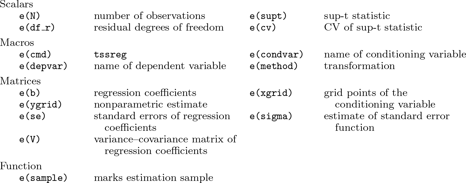
3.3 Stored results

tssreg stores the following in e():

4 Illustration of the method

4.1 Basic applications

A basic application of the tssreg command is to conduct a sup-t test for the conditional moment restriction

$E(Y_t|X_t=x)=0\text{ for}\hspace{0.17em}x\in \chi$

where χ is the observed support of X_t . In dynamic stochastic equilibrium models, this restriction can be derived from the martingale-difference property of the Y series with respect to an information filtration, according to Euler or Bellman equations in the structural model. Hence, under the null hypothesis, we can compute standard errors without accounting for autocorrelations of error terms. This can be done using the default option lag(0).

To illustrate, we use the dataset from the empirical study of Li and Liao (Forthcoming). data.dta contains three variables: timevar is the time index, the conditioning variable x is productivity, and the dependent variable y is generated according to the equilibrium conditions of a standard search-and-matching model. We set up the timeseries structure ¹ using tsset (see [TS] tsset), and then implement the sup-t test as follows:

With the default options, we carry out the test by nonparametrically fitting y using a fifth-order Legendre polynomial of the rank-transformed x. As shown in the table above, Stata reports the value of the sup-t statistic as 11.1841, which is far above the 5% CV. ² The p-value is virtually 0, suggesting a strong rejection of the hypothesis that E(y | x) = 0; that is, the equilibrium condition is not compatible with observed data.

Furthermore, if we use the table option, tssreg also reports the regression coefficients and the associated sampling information. For example,

Another important use of the tssreg command is to nonparametrically estimate the conditional expectation function h(x) = E(Y_t|X_t = x) and its uniform confidence band. The corresponding result can be visualized using the plot option and is presented as figure 1.

Figure 1.

Nonparametric fit and uniform confidence band without heteroskedasticityand autocorrelation-consistent estimation

We stress that the confidence band plotted in figure 1 is uniformly valid over the support of the conditioning variable displayed on the horizontal axis. In this example, the 95% confidence band does not always cover 0, suggesting that the conditional expectation function deviates from 0 at the 5% significance level. This finding is consistent with the aforementioned testing result. The figure also reveals that the rejection mainly occurs over the region where x is low.

When computing standard errors, the default setting lag(0) only accounts for conditional heteroskedasticity, ignoring all autocorrelations. This is appropriate if the error term Y_t − E(Y_t|X_t ) forms a martingale-difference sequence, which typically holds under the null hypothesis that the dynamic equilibrium model is correctly specified. However, if the empirical goal is to make a uniform inference on the conditional expectation function x ↦ E(Y_t|X_t = x), one should generally take into account time-series dependence by properly setting the lag parameter in the Newey–West estimator, analogous to the application of Stata’s built-in newey command (see [TS] newey). The following implementation sets the Newey–West lag parameter to 5 (and we also set the confidence level to 99% to illustrate the use of the confidencelevel() option). The resulting nonparametric estimate and confidence band are displayed in figure 2.

Figure 2.

Uniform confidence band with user-specified Newey–West lag parameter and confidence level

4.2 Choice of approximating functions

Series estimation involves choosing approximating functions and the number of series terms. While the default setting of tssreg provides a reasonable benchmark, applied users are encouraged to experiment with alternative specifications to check the robustness of their empirical findings with respect to these choices. In the current version, the approximating functions are constructed as Legendre polynomials of the transformed conditioning variable, where the specific transformation is set through the method() option. Legendre polynomials are orthogonal on the [−1, 1] interval. With a proper transformation, the distribution of the transformed conditioning variable can be made close to uniform on [−1, 1], which mitigates the issue of multicollinearity when many series terms are included in the regression.

Four types of transformations are available in the current version: affine, normal, lognormal, and rank. The common idea is first to fit the distribution of X_t , parametrically or nonparametrically, and then to use the fitted distribution function to transform the conditioning variable into a uniform distribution. Specifically, the options affine, normal, and lognormal correspond to parametrically fitting uniform, normal, and lognormal distributions, respectively. The default rank option implements a nonparametric transformation using the ranks (or, equivalently, the empirical distribution function) of the observed X_t data. The user can also use untransformed data by explicitly setting the method(none) option.

The number of series terms is determined by the m( # ) option. The constant term is always included. Hence, m( # ) corresponds to a (#–1)-order Legendre polynomial. Recall that a fifth-order Legendre polynomial is fit under the default setting.

As an example, we can examine the sensitivity of the empirical findings in the running example with respect to these choices. Sensitivity analysis like this is often needed in empirical work. We experiment with three transformations affine, normal, and rank. In addition, besides the default fifth-order Legendre polynomial, we also fit an eighth-order Legendre polynomial by using the m(9) option. The resulting plots are collected in figure 3.

Figure 3.

Nonparametric estimates and uniform confidence bands using different series approximations. Estimation in the top (respective bottom) row is conducted using 6 (respective 9) series terms. The left, middle, and right columns are generated using the affine, normal, and rank transformations, respectively. Individual graphs are combined using the grc1leg command (Wiggins 2010).

In all implementations, the null hypothesis E(Y_t|X_t ) = 0 is strongly rejected as before. Figure 3 also shows that essential features of the nonparametric estimation are robust with respect to the choice of approximating function and series terms.

4.3 Partial linear model and additional control variables

tssreg also accommodates additional control variables in a partially linear model:

$Y_t=h(X_t)+\beta \prime Z_t+{\epsilon }_t$

where Z _t is a list of control variables that are collected in controlvar. With these control variables, tssreg tests the null hypothesis

$h(x)=0\text{ all}\hspace{0.17em}x\in \chi$

and the plot option will display the nonparametric estimate and the uniform confidence band of the h(·) function. The table option reports regression coefficients of all series terms of X_t and control variables.

To illustrate, we include two randomly generated variables, z1 and z2, as controlvar in the running example. The results are displayed below.

Figure 4.

Nonparametric estimate and uniform confidence band with additional controls

Not surprisingly, because the additional control variables are in fact irrelevant in this example, the testing result remains the same, and the nonparametric estimates displayed in figure 4 are very close to those in figure 1.

4.4 Additional options

The ngrid() option sets the number of grid points used to discretize the support of X_t . Discretization is needed to compute the sup-t statistic, which is theoretically defined as the supremum over the support of the conditioning variable. The default is ngrid(100). Setting this parameter to a higher level reduces the approximation error from the discretization, while adding computational cost.

The trim() option allows the user to restrict the index set χ over which the sup-t statistic is computed. Specifically, trim( # ) restricts χ as [Q#/2, Q1−#/2], where Q_q is the q quantile of X_t . This option is useful if one’s empirical goal is to make a uniform inference only over the restricted region. Note that the underlying nonparametric series estimation is always based on all available data, whereas the trimming only affects the computation of the sup-t statistic and its CV.

The mc() option sets the number of simulations used to compute the CV. The default is mc(5000), which is adequate in most empirical contexts. The user may increase this number to improve the Monte Carlo approximation accuracy or decrease this number to reduce computation time.

The excel option saves information for reconstructing the nonparametric plots like figure 1. The output Excel file contains four columns: grid points of the conditioning variable, fitted values of the conditional expectation function, and lower and upper confidence bands at the user-specified confidence level.

Supplemental Material

Supplemental Material, st0614 - Uniform nonparametric inference for time series using Stata

Supplemental Material, st0614 for Uniform nonparametric inference for time series using Stata by Jia Li, Zhipeng Liao and Mengsi Gao in The Stata Journal

References

1.
AndrewsD. W. K.1991. Asymptotic normality of series estimators for nonparametric and semiparametric regression models. Econometrica59: 307–345. https://doi.org/10.2307/2938259.
2.
BelloniA.ChernozhukovV.ChetverikovD.KatoK.2015. Some new asymptotic theory for least squares series: Pointwise and uniform results. Journal of Econometrics186: 345–366. https://doi.org/10.1016/j.jeconom.2015.02.014.
3.
ChenX.2007. Large sample sieve estimation of semi-nonparametric models. In Handbook of Econometrics, vol. 6B, ed. HeckmanJ. J.LeamerE. E., 5549–5632. Amsterdam: Elsevier. https://doi.org/10.1016/S1573-4412(07)06076-X.
4.
ChenX.ChristensenT. M.2015. Optimal uniform convergence rates and asymptotic normality for series estimators under weak dependence and weak conditions. Journal of Econometrics188: 447–465. https://doi.org/10.1016/j.jeconom.2015.03.010.
5.
JannB.2005. moremata: Stata module (Mata) to provide various functions. Statistical Software Components S455001, Department of Economics, Boston College. https://ideas.repec.org/c/boc/bocode/s455001.html.
Please find the following supplemental material available below.
For Open Access articles published under a Creative Commons License, all supplemental material carries the same license as the article it is associated with.
For non-Open Access articles published, all supplemental material carries a non-exclusive license, and permission requests for re-use of supplemental material or any part of supplemental material shall be sent directly to the copyright owner as specified in the copyright notice associated with the article.