Sage Journals: Discover world-class research

Abstract

A few years ago, we developed metaan, a package to perform fixedor random-effects meta-analysis. In terms of random-effects meta-analysis, it offered a wide choice of models, including maximum likelihood, profile likelihood, or restricted maximum-likelihood, in addition to the established DerSimonian–Laird method available in metan or Cochrane’s RevMan software. Other unique features included a wide range of reported heterogeneity measures and a plot of the maximum likelihood function. Since then, metaan has been continuously updated to offer improved graphics, more options, and more meta-analysis models. In this necessary update, we describe these additions and discuss the new models and the evidence behind them.

Keywords

st0201_1 metaan meta-analysis random effects fixed effect effect sizes DerSimonian–Laird maximum likelihood profile likelihood restricted maximum likelihood Peto Mantel–Haenszel permutation(s) method bootstrap DerSimonian–Laird proportions forest plot

1 Introduction

Meta-analysis is a statistical methodology that combines the results of several independent studies, clinical trials or observational, that are considered appropriate to combine (Huque 1988). Traditionally, the term “meta-analysis” refers to pairwise meta-analysis of aggregate data. Pairwise implies a two-arm comparison, usually an intervention and a control arm, as opposed to the more recently developed network meta-analysis methods (Lumley 2002; Salanti, Ades, and Ioannidis 2011). Aggregate implies pooling reported results, usually in research articles, and involves extracting data on effects (or associations) and their variability, as opposed to the more challenging but also more promising individual patient data meta-analysis (Riley, Lambert, and Abo-Zaid 2010). Meta-analysis of aggregate data methodology focuses on the second step of a two-step process, the “pooling” of the extracted summary statistics into a weighted average, with the metaan and metan packages in Stata, dealing with pairwise analyses (Harris et al. 2008; Kontopantelis and Reeves 2010). A new set of commands, meta, is also available in Stata 16, offering a comprehensive approach with advanced meta-analysis methods. In R (R Core Team 2018), the metafor package offers a comprehensive suite of meta-analysis methods, including numerous random-effects approaches (Viechtbauer 2010), while meta is a user-friendly package that includes everything a meta-analyst would need as standard (Schwarzer 2007). Meta-analyses can also be conducted in SAS, but the process can be more challenging (Arthur, Bennett, and Huffcutt 2001). Specialist free software also exists, like RevMan, which is widely used in Cochrane reviews (Nordic Cochrane Centre 2007), but also easy-to-use Microsoft Excel add-ons like MIX (Bax et al. 2006) and MetaEasy (Kontopantelis and Reeves 2009b), which offer access to advanced meta-analysis methods through a widely available software platform. Specialist commercial software is also available, like CMA (Borenstein, Rothstein, and Cohen 2005). Older comparisons and overviews of available software exist, but this is a fast-moving field (Bax et al. 2007; Sterne, Egger, and Sutton 2001).

Arguably the biggest threats to meta-analysis, particularly meta-analysis of aggregate data, are publication bias and heterogeneity. Publication bias is extremely difficult to identify and address convincingly, with methods to identify it being underpowered in small meta-analyses (Sterne, Gavaghan, and Egger 2000) and methods to account for it requiring strong assumptions, thus making them contentious. For example, the intuitive and widely used trim-and-fill method (Duval and Tweedie 2000) fails to account for funnel-plot asymmetry that could be due to heterogeneity and thus can be too conservative (Peters et al. 2007). Heterogeneity, or between-study variance, is also difficult to reliably identify and stems from differences in populations, interventions, outcomes, follow-up times (clinical heterogeneity), or differences in trial design and quality (methodological heterogeneity) (Higgins and Thompson 2002; Thompson 1994). The difficulty in quantifying heterogeneity, as with publication bias, primarily relates to the small size of a typical meta-analysis and the fact that the underlying methods are asymptotic and work well with large study numbers.

How to appropriately address heterogeneity is another key validity issue. Fixedeffects models will not account for identified heterogeneity, assuming a single “true” effect, and thus limit the generalizability of the findings to the pooled studies. Randomeffects models will incorporate identified heterogeneity by assuming multiple “true” effects (some will assume they are normally distributed as well) and are typically more conservative and allow generalization. Considering that in the presence of heterogeneity, the performance of a fixed-effects approach deteriorates rapidly (Brockwell and Gordon 2001) and that random-effects models are robust even when the “true” effects deviate from normality (Kontopantelis and Reeves 2012a,b), we think that heterogeneity should always be modeled for the results to be generalizable–at any level and not only when above a certain arbitrary threshold (for example, I ² > 50% as is sometimes the case). Although methods to model heterogeneity are robust, the underlying problem is how to accurately estimate existing heterogeneity. Although homogeneity has been found to be the exception rather than the rule and some degree of “true” effect variability between studies is to be expected (Thompson and Pocock 1991), unobserved heterogeneity is a real problem, especially for meta-analyses of a few studies that tend to be the norm (Kontopantelis, Springate, and Reeves 2013).

To estimate heterogeneity, the standard approach is the method proposed by DerSimonian and Laird (1986), which has been widely implemented and is the default random-effects approach in generic and specialist meta-analysis statistical software. However, the between-study variance component can be estimated using alternative approaches, including iterative or nonparametric methods. These include maximum likelihood, profile likelihood, restricted maximum likelihood (REML) (Hardy and Thompson 1996; Thompson and Sharp 1999), and the nonparametric “permutations” method proposed by Follmann and Proschan (1999). A nonparametric bootstrap of the DerSimonian– Laird (DL) estimator was also shown to be a better performer, especially in small metaanalyses that were falsely assumed to be homogeneous under the standard DL model (Kontopantelis, Springate, and Reeves 2013), and that was recently verified in a more complete and independent simulation comparison (Petropoulou and Mavridis 2017). Because of the difficulty in detecting underlying heterogeneity in small meta-analyses and inaccurate estimates, sensitivity analyses using a range of heterogeneity levels have also been recommended (Kontopantelis, Springate, and Reeves 2013). Small meta-analyses are also more likely to end up with a sample of studies that is not representative, which can result in incorrect estimates of true heterogeneity.

We have implemented all these methods in metaan, offering numerous alternatives to the DL random-effects model. Since the first appearance of metaan, we have been continuously updating it, and the latest version offers improved graphics, dichotomous outcomes analyses, and more meta-analysis models. Besides the standard fixed-effects model, we have also implemented the Mantel–Haenszel and Peto methods for dichotomous outcomes (Greenland and Robins 1985; Yusuf et al. 1985), which have been shown to perform well for rare and very rare events, respectively (Bradburn et al. 2007). The command requires the study-specific estimates and standard errors, or arm-specific event and nonevent counts, for each study to be meta-analyzed. A complementing command, metaeff (Kontopantelis and Reeves 2009a), can be used to calculate the effect size and its standard error from the input parameters supplied by the user for each study, using one of the methods described in the Cochrane Handbook for Systematic Reviews of Interventions (Higgins and Green 2011; Kontopantelis and Reeves 2009b). The metaan command can also perform stratified meta-analysis and meta-analysis of proportions with the Freeman–Tukey arcsine transformation as well as provide elaborate forest plots using the dispgby package and likelihood plots for estimates obtained from the maximum likelihood models. Numerous measures of heterogeneity and their confidence intervals are also reported, including I ² (0 to 100% range), H ² (≥ 1), and the between-study variance estimate ${\hat{τ}}^{2}$ (Higgins and Thompson 2002; Mittlböck and Heinzl 2006). In the following sections, we describe these additions through several examples.

2 The metaan command

2.1 Updates to metaan

Since metaan first appeared in 2010, we have added numerous features. We felt that these additions necessitated this article to serve as a more comprehensive guide for users, compared with the command’s help file. Major additions included the following:

February 25, 2013: new meta-analysis models, bootstrap DL, and sensitivity analysis using preset values for I ².

August 14, 2014: dealing with proportions with the Freeman–Tukey transformation.

September 5, 2014: support for α level other than 5%; reporting confidence intervals for heterogeneity measures.

September 18, 2014: support for back-transforming effects to odds ratios (ORs) for binary outcomes.

June 20, 2015: major update for forest plot to use program dipgby by Ross Harris and Mike Bradburn (same program used by metan).

April 11, 2016: by option added for subgroup analyses.

July 25, 2018: added support for binary data with all commonly used methods (Mantel–Haenszel, Peto, or inverse variance), with a new four-variable syntax.

September 10, 2018: added back-transformation for meta-analyses of log-transformed effects.

Details on all these additions, along with the original capabilities and options for the command are described in detail below.

2.2 Description

The metaan command performs a meta-analysis on a set of studies and estimates the overall effect µ and its confidence interval. The command also displays various heterogeneity measures: Cochrane’s Q, I ² (in the [0, 100%) range with larger scores indicating higher levels of heterogeneity), H ² (equals 1 in the case of homogeneity), and the between-study variance (τ ²) estimate. Cochrane’s Q is the same across all methods, but the between-study variance estimate (and hence I ² and H ²) can vary between the DL (dl) and maximum likelihood (ml) methods. Only one method option must be selected, with the exception of the four methods for event data: Mantel–Haenszel OR (mhor), Mantel–Haenszel risk ratio (mhrr), Mantel–Haenszel risk difference (mhrd), and Peto OR (por). Each one of these four approaches for binary data can be combined with the other models for different weighting and random-effects options. For calculating the effects and variance of the effects for a group of studies from various statistical parameters, please see the package metaeff. The command will automatically detect the alpha level in the environment and use it (edit by typing set level 99, for example).

The command requires the user to first specify either two or four variable names. When only two are specified, metaan assumes these refer to study effects and standard errors; when four are specified, the command assumes they represent study-group specific event and nonevent counts for a binary outcome. When the study effects and standard errors are specified, metaan uses the standard fixed-effects model or one of many inverse-variance weighting methods to account for heterogeneity. Binary and continuous outcomes can be implemented using this syntax, provided the effect and its variability are available. In this case, the command expects as input the log() of the measure (OR, risk ratio, or hazard ratio [HR]) in varname1 and its standard error in varname2 (see appendix tables in Kontopantelis and Reeves [2009b] regarding relevant methods, which are available in metaeff). The default output is then the overall log() of the measure unless the user specifies the exp option, which returns the exponentiated results (to ORs, risk ratios, HRs, etc.). The name of the measure can be input with the forest plot option effect(), the default being OR.

When group-specific event and nonevent counts are specified, metaan calls Mantel– Haenszel and Peto fixed-effects meta-analysis methods for binary outcomes. These methods necessarily ignore heterogeneity but have been shown to work well in rare (Mantel–Haenszel) and very rare (Peto) event settings—where heterogeneity is difficult to measure anyway. Three Mantel–Haenszel approaches are provided, in terms of the effect calculation: OR, risk ratio, and risk difference. The Peto “OR” is not really an OR, but it has come to be known as that. For the Mantel–Haenszel approaches, zero-cell corrections are applied. Corrections are not needed for Peto because of the way the effects are calculated. Weightings with these approaches differ from standard inverse-variance weighting and are closer, but not the same, to fixed-effects weighting, where the size of the study is the primary determinant (Peto uses an inverse-variance approach but different weights and a different estimand). Each of these four methods can be combined with any of the inverse-variance models or the fixed-effects approach. In that case, the effect and its variance are calculated using the respective method for event data (one of mhor, mhrr, mhrd, or por), which is then meta-analyzed. This approach allows for modeling heterogeneity, but the weighting can be different, as previously mentioned (these “hybrid” methods are provided in Cochrane’s RevMan). The command always meta-analyzes the ORs and risk ratios on the log() scale and, by default, returns results on that scale. Users can specify the exp option to obtain exponentiated results of these (note that risk difference is not a ratio and the log() scale and the exp option do not apply).

For meta-analyses of time-to-event outcomes, the use of adjusted HRs is advised with the two-variable syntax. A reasonable alternative is the calculation of the log HR from a log-rank analysis. The log HR is estimated by (O − E)/V , which has standard error $1 / \sqrt{V}$ , where O is the observed number of events on the intervention, E is the log-rank expected number of events on the intervention, O − E is the log-rank statistic, and V is the variance of the log-rank statistic. The Peto method can also be used in this context, because it is O − E based, to pool HRs (or ORs) with option poe, which is equivalent to a fixed-effects approach. Dichotomous data approaches (mhor, mhrr, mhrd, or por) are not advised here even if the follow-up times are identical across studies, because these methods cannot account for censored data.

2.3 Syntax

metaan varname1 varname2 [varname3 varname4] [if] [in] [, fe dl bdl ml reml pl pe sa poe mhor mhrr mhrd por grpby( varname ) label( varlist ) varc prp exp backt( varlist ) pscl reps( # ) seed( # ) sens( # ) plplot( string ) forest ]

Two syntaxes are possible. In the first, the user is expected to provide varname1 and varname2 only, which include information on study-effect sizes and study-effect variation (the default being standard error/deviation), respectively. If the prp option is selected for meta-analysis of proportions, varname1 and varname2 should hold numerators and denominators, respectively. The second syntax is used for binary outcomes with event data, and four variables are expected, with varname1 being the number of events in group 1, varname2 the number of nonevents in group 1, varname3 the number of events in group 2, and varname4 the number of nonevents in group 2.

2.4 Options

Meta-analysis model

fe fits a fixed-effects model that assumes there is no heterogeneity between the studies. The model assumes that within-study variances may differ but that there is homogeneity of effect size across all studies. Often, the homogeneity assumption is unlikely, and variation in the true effect across studies is to be expected. Therefore, caution is required when using this model. Reported heterogeneity measures are estimated using the inverse-variance weighting and the DL model.

dl fits a DL random-effects model, which is the most commonly used model. The model assumes heterogeneity between the studies; that is, assumes that the true effect can be different for each study. The method assumes that the individual-study true effects are distributed with a variance τ ² around an overall true effect but makes no assumptions about the form of the distribution of either the within-study or the between-study effects. Inverse-variance weighting is used as opposed to fixed-effects weighting, which is based on study size, and small studies may be given disproportionally large weights. Reported heterogeneity measures are estimated using the DL model.

bdl fits a bootstrap DL model, which is similar to DL but better performing, especially for small meta-analyses. It uses a nonparametric bootstrap to estimate the between-study variance and other heterogeneity parameters. Reported heterogeneity measures are estimated using the bootstrap DL model.

ml fits a maximum-likelihood random-effects model. This model makes the additional assumption (necessary to derive the log-likelihood function and also true for reml and pl below) that both the within-study and the between-study effects are normally distributed. It solves the log-likelihood function iteratively to produce an estimate of the between-study variance. However, the method does not always converge; in some cases, the between-study variance estimate is negative and set to zero, in which case the model is reduced to the fe specification. Estimates are reported as missing in the event of nonconvergence. Reported heterogeneity measures are estimated using the maximum likelihood model.

reml fits an REML random-effects model. This model is similar to ml and uses the same assumptions. The log-likelihood function is maximized iteratively to provide estimates as in ml. However, under reml, only the part of the likelihood function that is location invariant is maximized (that is, maximizing the portion of the likelihood that does not involve µ if estimating τ ², and vice versa). The method does not always converge; in some cases, the between-study variance estimate is negative and set to zero, in which case the model is reduced to the fe specification. Estimates are reported as missing in the event of nonconvergence. Reported heterogeneity measures are estimated using the REML model.

pl fits a profile-likelihood random-effects model. This model uses the same likelihood function as ml but accounts for the uncertainty associated with the between-study variance estimate when calculating an overall effect, which is done using nested iterations to converge to a maximum. The confidence intervals provided by the method are asymmetric and hence so is the diamond in the forest plot. However, the method does not always converge. Values that were not computed are reported as missing. Reported heterogeneity measures are estimated using the maximum likelihood model (the effect µ and τ ² estimates are the same; only the confidence intervals are reestimated) but also provide a confidence interval for the between-study variance estimate.

pe fits a permutations random-effects model. This is a nonparametric random-effects method, which can be described in three steps. First, in line with a null hypothesis that all true study effects are zero and observed effects are due to random variation, a dataset of all possible combinations of observed study outcomes is created by permuting the sign of each observed effect. Then, the DL method is used to compute an overall effect for each combination. Finally, the resulting distribution of overall effect sizes is used to derive a confidence interval for the observed overall effect. The confidence interval provided by the method is asymmetric and hence so is the diamond in the forest plot. Study weights and heterogeneity measures are estimated using the DL model.

sa fits a sensitivity analysis model. This allows sensitivity analyses to be performed by varying the level of heterogeneity, with I ² taking values in the [0, 100) range. Undetected heterogeneity is the norm rather than the exception, and we encourage users to test the sensitivity of their results in the presence of moderate (50%) and high (80–90%) levels of heterogeneity (please see Kontopantelis, Springate, and Reeves [2013]). Reported heterogeneity measures are based on the preset I ² level.

poe fits a Peto fixed-effects approach for time-to-event O−E (observed minus expected) data. By default, the log() of HRs is assumed to be provided for meta-analysis, which can be exponentiated to HRs with the exp option. ORs can also be meta-analyzed [again, expecting log(OR) as input and the variance of the effect]; in this case, if a forest plot is requested, the outcome label should be edited with the effect() option. The method is identical to fe and is provided only for completeness and clarity.

Binary outcome data with group-specific event and nonevent counts

mhor fits a Mantel–Haenszel fixed-effects model with effect calculation based on OR. It can be combined with inverse-variance models to account for heterogeneity or a fixed-effects model, for different weighting approaches. If a random-effects or fixed-effects approach is used in combination with the mhor option, weighting follows the random-effects or fixed-effects approach used, and Mantel–Haenszel is relevant only in the way the effect is calculated within each study from events and nonevents. The exp option needs to be used to report effects as ORs and not on the log() scale.

mhrr fits a Mantel–Haenszel fixed-effects model with effect calculation based on risk ratio (RR). It can be combined with inverse-variance models to account for heterogeneity or a fixed-effects model, for different weighting approaches. If a random-effects or fixed-effects approach is used in combination with the mhrr option, weighting follows the random-effects or fixed-effects approach used, and Mantel–Haenszel is relevant only in the way the effect is calculated within each study from events and nonevents. The exp option needs to be used to report effects as RRs and not on the log() scale.

mhrd fits a Mantel–Haenszel fixed-effects model with effect calculation based on riskdifference. It can be combined with inverse-variance models to account for heterogeneity or a fixed-effects model for different weighting approaches. If a randomeffects or fixed-effects approach is used in combination with the mhrd option, weighting follows the random-effects or fixed-effects approach used, and Mantel–Haenszel is relevant only in the way the effect is calculated within each study from events and nonevents.

por fits a Peto OR fixed-effects model. It can be combined with inverse-variance models to account for heterogeneity or a fixed-effects model for different weighting approaches. In that case, the por option is relevant only to the effect calculation (which is technically not an OR, but the name has stuck). The exp option needs to be used to report effects as ORs and not on the log() scale.

General modeling options

grpby( varname ) specifies the grouping variable for subgroup analyses. An integer numeric variable is expected, ideally with appropriate value labels; see [D] label. The groups will be ordered according to the variable provided, and headers for the results and the forest plot (if requested) will be obtained from the variable’s value labels (if no labels are present, the relevant numbers will be used). All analyses are repeated for each group category and overall. Results are presented as separate analyses in the Results window but are all aggregated into a single forest plot (if one is requested).

label( varlist ) selects labels for the studies. One or two variables can be selected and converted to strings. If two variables are selected, they will be separated by a comma. Usually, the author names and the year of study are selected as labels. The final string is truncated to 20 characters.

varc specifies that the study-effect variation variable, varname2, holds variance values. If this option is omitted, metaan assumes the variable contains standard-error values (the default).

prp specifies that numerators (varname1) and denominators (varname2) are provided and a meta-analysis of proportions will be executed. The Freeman–Tukey arcsine transformation is used, variance is calculated as 1/(varname2 + 1), and effects and confidence intervals (study and overall) are back-transformed using {sin(x/2)}².

exp specifies that the results will be exponentiated for dichotomous outcomes. For dichotomous outcomes, the log() of the measure (OR, RR, or HR) and its standard error are expected as input and the overall log() of the measure is returned by default unless this option is specified. If it is, the input is still expected to be the log() of the measure in varname1, but results are exponentiated.

backt( varlist ) specifies the back-transformation to percentages, from simple or empirical logit (Stevens et al. 2016). One or two variables can be selected. The first holds the study “anchor” percentages, which are essential for the back-transformation to take place. The second holds the relevant denominators. If only percentages are provided, they need to be in the (0, 1) range for back-transformation from simple empirical logit. However, if any zeros or ones are present in the percentages variable, the empirical logit will need to be used, and in this case the denominators are needed as well. The overall effect is back-transformed using the mean percentage across all studies as the “anchor”. If denominators are provided, then the mean percentage is weighted on denominators; if not, it is unweighted.

pscl scales to [0%–100%] when using the prp or backt() option. The default display for percentages in the output and forest plot is in the [0, 1] range.

Bootstrap DerSimonian–Laird options

reps( # ) specifies the integer number of repetitions for the bootstrap DL method. Fewer than 100 repetitions are not permitted.

seed( # ) specifies the random-number seed to be used in the bootstrap DL method.

Sensitivity analysis options

sens( # ) specifies the preset heterogeneity level, with I ² taking values in the [0, 100) range. The default is sens(80).

Graphs

Only one graph output is allowed in each execution.

plplot( string ) requests a plot of the likelihood function for the µ or τ ² estimates of the ml, pl, or reml model. The plplot(mu) option fixes µ to its model estimate in the likelihood function and creates a two-way plot of τ ² versus the likelihood function. The plplot(tsq) option fixes τ ² to its model estimate in the likelihood function and creates a two-way plot of µ versus the likelihood function.

forest requests a forest plot. The weights from the specified analysis are used for plotting symbol sizes. Since version 2.0 of the command, we use the _dispgby program by Ross Harris and Mike Bradburn, which is integrated with other popular meta-analysis commands (for example, metan). We allow all relevant options (see below).

Forest plot options

Various graph options can be used to specify overall graph options that would appear at the end of a twoway command. This allows the addition of titles, subtitles, captions, etc.; it also allows control of margins, plot regions, graph size, aspect ratio, and the use of schemes. Specific options are listed below.

dp( # ) specifies the decimal points for the reported effects. The default is dp(2).

effect( string ) allows the graph to name the summary statistic used [for example, OR, RR, standardized mean difference (SMD)].

favours( string # string ) applies a label saying something about the treatment effect to either side of the graph (strings are separated by the # symbol).

null( # ) displays the null line at a user-defined value rather than 0 or 1.

nulloff removes the null hypothesis line from the graph.

noverall prevents display of overall effect size on the graph (automatically enforces the nowt option).

nowt prevents display of study weights on the graph.

nostats prevents display of study statistics on the graph.

nowarning switches off the default display of a note warning that studies are weighted from random-effects analyses.

nohet prevents display of heterogeneity statistics in the graph.

nobox prevents a weighted box from being drawn for each study, and only markers for point estimates are shown.

boxsca( # ) controls box scaling. The default is boxsca(100) (as in a percentage) and may be increased or decreased as such (for example, 80 or 120 for 20% smaller or larger, respectively).

xlabel( numlist ) defines x-axis labels. Any number of points may be defined, and the range can be enforced with the use of the force option. Points must be comma separated.

xtick( numlist ) adds tick marks to the x axis. Points must be comma separated.

force forces the x-axis scale to be in the range specified by xlabel().

textsize( # ) specifies font size for the text display on the graph. The default is textsize(100) (as in a percentage) and may be increased or decreased as such (for example, 80 or 120 for 20% smaller or larger, respectively).

astext( # ) specifies the percentage of the graph to be taken up by text. The default is astext(50), and the percentage must be in the range [10, 90].

summaryonly shows only summary estimates in the graph.

classic specifies that solid black boxes without point estimate markers are used as in previous versions.

lcols( varlist ) and rcols( varlist ) define columns of additional data to the left or right of the graph. The first two columns on the right are automatically set to effect size and weight unless suppressed using the options nostats and nowt. textsize() can be used to fine-tune the size of the text to achieve a satisfactory appearance. The columns are labeled with the variable label or the variable name if the label is not defined. The first variable specified in lcols() is assumed to be the study identifier, and this is used in the table output.

double allows variables specified in lcols() and rcols() to run over two lines in the plot. This may be of use if long strings are to be used.

boxopt( options ), diamopt( options ), pointopt( options ), ciopt( options ), and olineopt( options ) specify options for the graph routines within the program, allowing the user to alter the appearance of the graph. Any options associated with a particular graph command may be used except some that would cause incorrect graph appearance.

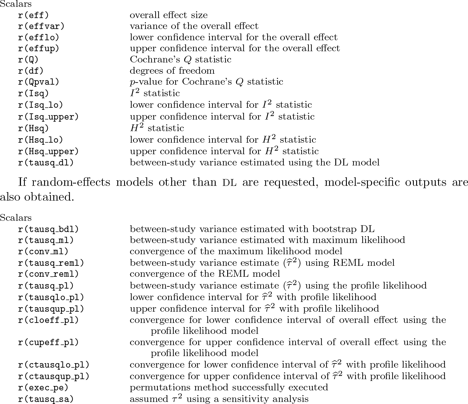
2.5 Stored results

metaan stores the following in r():

3 Examples

We provide a few examples with the two-and four-variable syntaxes to give users a better understanding of the required data and the analysis options.

3.1 Meta-analysis based on effects and their standard errors

Let us assume an artificial dataset of 11 studies with information on a particular intervention, for example, a specific psychological intervention to reduce depression levels in populations diagnosed with severe depression in primary care. Let us also assume that various scales to quantify depression levels have been used across these studies and we have collected data on the mean difference in depression levels between the intervention and control group, six months following the intervention. In other words, for study i, we have the mean difference MD _i = MNa6 _Ai − MNa6 _Bi , where MNa6 _Ai and MNa6 _Bi are the mean depression levels in study i, six months postintervention, for the intervention (A) and control (B) groups, respectively. Assuming the studies are randomized controlled trials, as they often are, available preintervention data points are not used because the groups should be well balanced. If there is no balance in the outcome preintervention, as in many observational studies, then the last available preintervention time point needs to be accounted for. For example, the mean difference would be MD _i = (MNa6 _Ai − MNb0 _Ai ) − (MNa6 _Bi − MNb0 _Bi ), where MNb0 _Ai and MNb0 _Bi are the mean depression levels in study i, just before the administering of the intervention, for the intervention (A) and control (B) groups, respectively. However, severely unbalanced group comparisons can be problematic for the validity of such analyses. Getting back to our example, we assume good preintervention group balance, but the outcome is measured across numerous scales (for example, BDI, CES-D, or PHQ-9). Therefore, we would need to calculate and meta-analyze the SMD for each study as ${SMD}_{i} = (M N a 6_{A i} - M N a 6_{B i}) / \sqrt{SD a 6_{A i}^{2} + SD a 6_{B i}^{2}}$ . We use the pooled variance in the postintervention time point that is the focus of our analysis (in this case, six months), with SDa6D_Ai and SDa6 _Bi denoting the standard deviation (SD) in study i, six months postintervention, for the intervention (A) and control (B) groups, respectively. In our example dataset below, variable eff is assumed to hold the SMD values, and variable SEeff the pooled SD values, or $\sqrt{SD a 6_{A i}^{2} + SD a 6_{B i}^{2}}$ .

First, we meta-analyze studies using a random-effects model and bootstrap DL estimator, with 1,000 repetitions.

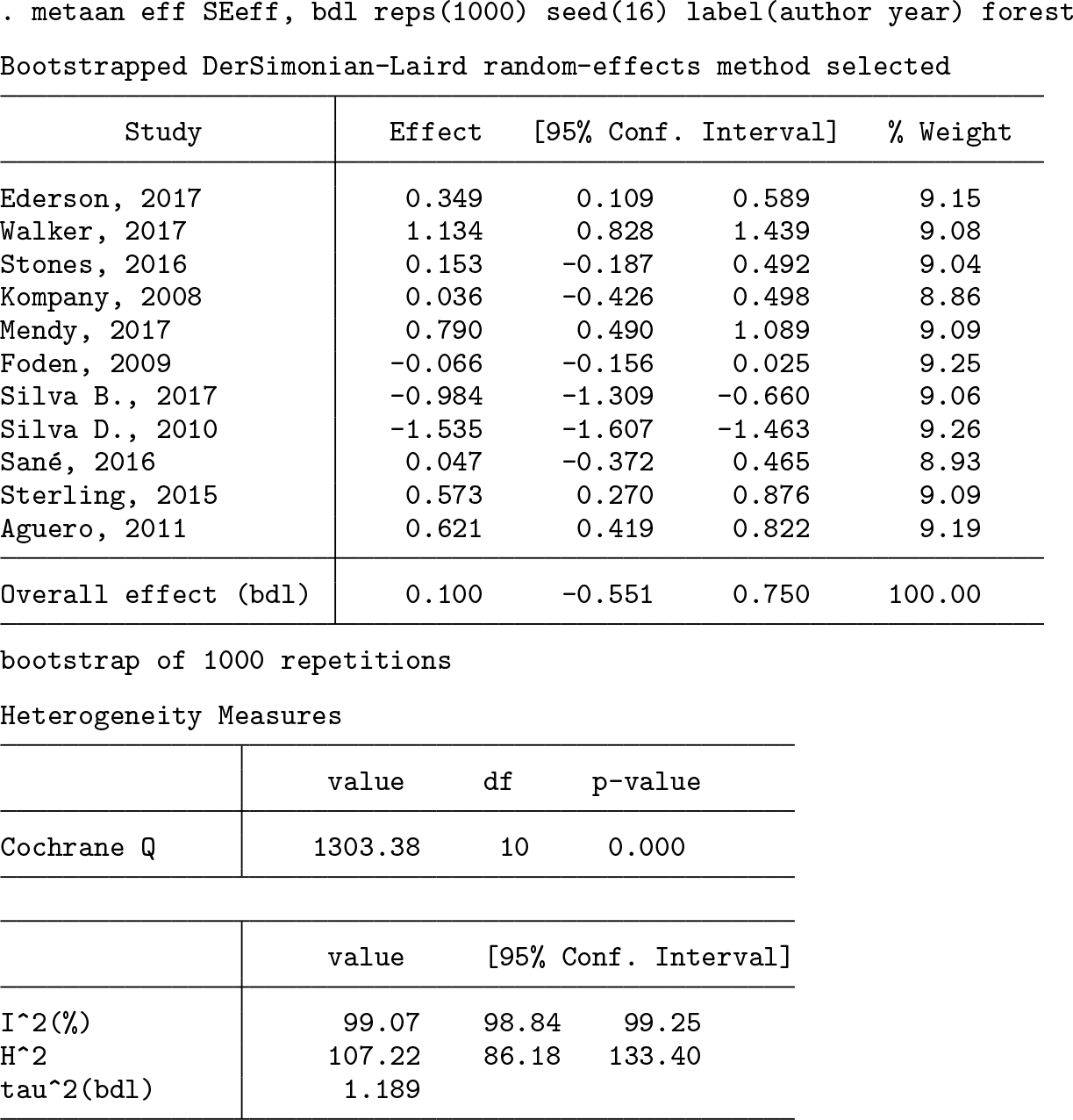
High levels of heterogeneity were observed and modeled. The overall effect is not statistically different from zero. Therefore, the conclusion would be that the overall effect of this hypothesized specific psychological intervention for severe depression is not statistically different from zero, although there was great variability in its effectiveness across included studies. Figure 1 shows the requested forest plot.

Figure 1.

Bootstrap DL random-effects model

Next, we meta-analyze studies using the profile-likelihood random-effects model and request a likelihood plot for the overall effect estimate $\hat{µ}$ .

Figure 2.

Likelihood plot for $\hat{µ}$

The heterogeneity estimates are similar to what we observed with the bootstrap DL model, as is the overall effect. Figure 2 shows the requested likelihood plot for $\hat{µ}$ . The profile likelihood method converged for all estimates and their confidence intervals.

3.2 Meta-analysis using event and nonevent counts

Let us assume that we are interested in treatment for heart attacks, particularly primary percutaneous coronary intervention. We hypothesize that the outcome of interest is five-year postoperative mortality and that there are no censored values (all patients are followed up for five years or until death). Our aim is to evaluate the role of a new blood-thinning medication, so we use a second dataset with events and nonevents for the binary outcome. Variable Ine is the number of operated cases who were administered the medication and survived, and Ie the number of deaths in that group. Similarly, variable Cne is the number of operated cases who were not administered the medication and survived, and Ce the number of deaths in that group.

First, we meta-analyze studies using a Peto OR fixed-effects model. Results are exponentiated, and a forest plot is requested.

We used the Peto fixed-effects approach (with Peto weighting), although heterogeneity was identified (under an inverse-variance approach). Assuming we are analyzing adverse events, the blood-thinning agent appears to have a modest prophylactic effect on five-year survival, which is also statistically significant. Figure 3 shows the requested forest plot.

Figure 3.

Peto fixed-effects model

Next, we account for heterogeneity using the bootstrap DL random-effects model with inverse-variance weighting. In the first step, we use the Mantel–Haenszel risk-ratio approach to calculate the effect size and its variance for each study.

When we account for heterogeneity, the overall effect is closer to 1.0 and not statistically significant. This is not surprising considering random-effects models are generally more conservative from incorporating between-study variability. Finally, we wish to examine how results would change if this sample of studies underrepresented actual heterogeneity. 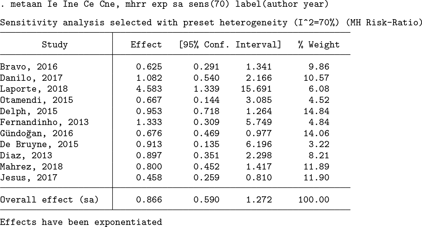For this, we use the sensitivity analysis model with a preset heterogeneity level of 70% (the upper limit of $\hat{I^{2}}$ in the previous model, though other values may be chosen).

Under this higher heterogeneity assumption, the overall effect is even more slightly reduced, though the greater impact is a wider confidence interval. This approach can be useful in evaluating how sensitive analyses are to undetected or underestimated heterogeneity, something rather common in small meta-analyses in particular.

4 Discussion

The metaan package for Stata was first published in 2010. Since then, we have incorporated numerous additions, particularly additional features for conducting random-effects meta-analysis. It is now an extensive meta-analysis package for binary, continuous, or prevalence (proportions) data, allowing numerous options and offering attractive graphical outputs. In this article, we have described and demonstrated many of the package’s capabilities and have highlighted the methodological evidence behind the implemented methods. Currently, unique to metaan are some of the best performing random-effects models like the nonparametric bootstrap DL, allowing users to potentially obtain more reliable results. Unique features also include the profile likelihood plot and the backtransformation options, while the heterogeneity sensitivity analysis was first presented in metaan and is now available in the built-in meta command from Stata 16. We need to highlight that meta, Stata’s new and comprehensive suite of meta-analysis commands, will be suitable for the needs of most users and includes advanced methods; for example, it does not use the DL estimator for its default random-effects model but instead uses restricted maximum-likelihood. However, metaan includes some unique features that would still make an attractive alternative, like the best-performing nonparametric bootstrap DL (Petropoulou and Mavridis 2017). In addition, it will serve well users of Stata 15 or previous, in which the meta suite of commands is not available. We will continue developing and updating metaan hand in hand with emerging best-practice evidence. The latest version is available from http://www.statanalysis.co.uk/.

Supplemental Material

Supplemental Material, st0201_1 - Pairwise meta-analysis of aggregate data using metaan in Stata

Supplemental Material, st0201_1 for Pairwise meta-analysis of aggregate data using metaan in Stata by Evangelos Kontopantelis and David Reeves in The Stata Journal

Footnotes

This study was partially funded by the National Institute of Health Research School for Primary Care Research through a personal fellowship for Evangelos Kontopantelis. The study represents independent research by the National Institute of Health Research. The views expressed in this publication are those of the authors.

Acknowledgments

We thank Mike Bradburn and Ross Harris, whose code helped shape the command.

Contributions

Evangelos Kontopantelis designed and developed the command and drafted the article. David Reeves critically commented on both the article and the functionality of the command.

Evangelos Kontopantelis and David Reeves declare no conflicts of interest.

5 Programs and supplemental materials

To install a snapshot of the corresponding software files as they existed at the time of publication of this article, type

The latest version of the command is available from . Within Stata, type

Alternatively, install from the Statistical Software Components archive, where updates are uploaded with a few days’ lag:

The data used in the examples are openly available from http://www.statanalysis. co.uk. From within Stata, to download the datasets in the current directory, type

References

Arthur

Jr Bennett

Jr Huffcutt

A. I.

2001. Conducting Meta-Analysis using SAS. New York: Psychology Press.

Bax

L.-M.

Ikeda

Moons

K. G. M.

2007. A systematic comparison of software dedicated to meta-analysis of causal studies. BMC Medical Research Methodology 7: 40. https://doi.org/10.1186/1471-2288-7-40.

Bax

L.-M.

Ikeda

Tsuruta

Moons

K. G. M.

2006. Development and validation of MIX: Comprehensive free software for meta-analysis of causal research data. BMC Medical Research Methodology 6: 50. https://doi.org/10.1186/1471-2288-6-50.

Borenstein

Rothstein

Cohen

2005. Comprehensive Meta-Analysis: A Computer Program for Research Synthesis. Englewood, NJ: Biostat.

Bradburn

M. J.

Deeks

J. J.

Berlin

J. A.

Localio

A. R.

2007. Much ado about nothing: A comparison of the performance of meta-analytical methods with rare events. Statistics in Medicine 26: 53–77. https://doi.org/10.1002/sim.2528.

Brockwell

S. E.

Gordon

I. R.

2001. A comparison of statistical methods for meta-analysis. Statistics in Medicine 20: 825–840. https://doi.org/10.1002/sim.650.

DerSimonian

Laird

1986. Meta-analysis in clinical trials. Controlled Clinical Trials 7: 177–188. https://doi.org/10.1016/0197-2456(86)90046-2.

Duval

Tweedie

2000. Trim and fill: A simple funnel-plot–based method of testing and adjusting for publication bias in meta-analysis. Biometrics 56: 455–463. https://doi.org/10.1111/j.0006-341X.2000.00455.x.

Follmann

D. A.

Proschan

M. A.

1999. Valid inference in random effects metaanalysis. Biometrics 55: 732–737. https://doi.org/10.1111/j.0006-341X.1999.00732.x.

10.

Greenland

Robins

J. M.

1985. Estimation of a common effect parameter from sparse follow-up data. Biometrics 41: 55–68. https://doi.org/10.2307/2530643.

11.

Hardy

R. J.

Thompson

S. G.

1996. A likelihood approach to meta-analysis with random effects. Statistics in Medicine 15: 619–629. https://doi.org/10.1002/(SICI)1097-0258(19960330)15:6h619::AID-SIM188i3.0.CO;2-A.

12.

Harris

R. J.

Bradburn

M. J.

Deeks

J. J.

Harbord

R. M.

Altman

D. G.

Sterne

J. A. C.

2008. metan: Fixedand random-effects meta-analysis. Stata Journal 8: 3–28. https://doi.org/10.1177/1536867X0800800102.

13.

Higgins

J. P. T.

Green

2011. Cochrane Handbook for Systematic Reviews of Interventions Version 5.1.0. http://www.cochrane-handbook.org.

14.

Higgins

J. P. T.

Thompson

S. G.

2002. Quantifying heterogeneity in a metaanalysis. Statistics in Medicine 21: 1539–1558. https://doi.org/10.1002/sim.1186.

15.

Huque

M. F.

1988. Experiences with meta-analysis in NDA submissions. Proceedings of the Biopharmaceutical Section of the American Statistical Association 2: 28–33.

16.

Kontopantelis

Reeves

2009a. metaeff: Stata module to perform effect sizes calculations for meta-analyses. Statistical Software Components S457072, Department of Economics, Boston College. https://ideas.repec.org/c/boc/bocode/s457072.html.

17.

Kontopantelis

Reeves

2009b. MetaEasy: A meta-analysis add-in for Microsoft Excel. Journal of Statistical Software 30(7): 1–25. https://doi.org/10.18637/jss.v030.i07.

18.

Kontopantelis

Reeves

2010. metaan: Random-effects meta-analysis. Stata Journal 10: 395–407. https://doi.org/10.1177/1536867X1001000307.

19.

Kontopantelis

Reeves

2012a. Performance of statistical methods for meta-analysis when true study effects are non-normally distributed: A comparison between DerSimonian–Laird and restricted maximum likelihood. Statistical Methods in Medical Research 21: 657–659. https://doi.org/10.1177/0962280211413451.

20.

Kontopantelis

Reeves

2012b. Performance of statistical methods for meta-analysis when true study effects are non-normally distributed: A simulation study. Statistical Methods in Medical Research 21: 409–426. https://doi.org/10.1177/0962280210392008.

21.

Kontopantelis

Springate

D. A.

Reeves

2013. A re-analysis of the Cochrane Library data: The dangers of unobserved heterogeneity in meta-analyses. PLOS ONE 8: e69930. https://doi.org/10.1371/journal.pone.0069930.

22.

Lumley

2002. Network meta-analysis for indirect treatment comparisons. Statistics in Medicine 21: 2313–2324. https://doi.org/10.1002/sim.1201.

23.

Mittlböck

Heinzl

2006. A simulation study comparing properties of heterogeneity measures in meta-analyses. Statistics in Medicine 25: 4321–4333. https://doi.org/10.1002/sim.2692.

24.

Nordic Cochrane Centre. 2007. Review Manager (RevMan): Version 5. Software program. Copenhagen: The Nordic Cochrane Centre, The Cochrane Collaboration.

25.

Peters

J. L.

Sutton

A. J.

Jones

D. R.

Abrams

K. R.

Rushton

2007. Performance of the trim and fill method in the presence of publication bias and betweenstudy heterogeneity. Statistics in Medicine 26: 4544–4562. https://doi.org/10.1002/sim.2889.

26.

Petropoulou

Mavridis

2017. A comparison of 20 heterogeneity variance estimators in statistical synthesis of results from studies: A simulation study. Statistics in Medicine 36: 4266–4280. https://doi.org/10.1002/sim.7431.

27.

R Core Team. 2018. R: A Language and Environment for Statistical Computing. R Foundation for Statistical Computing, Vienna, Austria. http://www.R-project.org.

28.

Riley

R. D.

Lambert

P. C.

Abo-Zaid

2010. Meta-analysis of individual participant data: Rationale, conduct, and reporting. British Medical Journal 340: c221. https://doi.org/10.1136/bmj.c221.

29.

Salanti

Ades

A. E.

Ioannidis

J. P. A.

2011. Graphical methods and numerical summaries for presenting results from multiple-treatment meta-analysis: An overview and tutorial. Journal of Clinical Epidemiology 64: 163–171. https://doi.org/10.1016/j.jclinepi.2010.03.016.

30.

Schwarzer

2007. meta: An R package for meta-analysis. R News 7: 40–45.

31.

Sterne

J. A. C.

Egger

Sutton

A. J.

2001. Meta-analysis software. In Systematic Reviews in Health Care: Meta-Analysis in Context, 2nd edition, ed. Egger

Davey Smith

Altman

D. G.

, 336–346. London: BMJ Books. https://doi.org/10.1002/9780470693926.ch17.

32.

Sterne

J. A. C.

Gavaghan

Egger

2000. Publication and related bias in meta-analysis: Power of statistical tests and prevalence in the literature. Journal of Clinical Epidemiology 53: 1119–1129. https://doi.org/10.1016/S0895-4356(00)00242-0.

33.

Stevens

Valderas

J. M.

Doran

Perera

Kontopantelis

2016. Analysing indicators of performance, satisfaction, or safety using empirical logit transformation. British Medical Journal 352: i1114. https://doi.org/10.1136/bmj.i1114.

34.

Thompson

S. G.

1994. Systematic review: Why sources of heterogeneity in metaanalysis should be investigated. British Medical Journal 309: 1351–1355. https://doi.org/10.1136/bmj.309.6965.1351.

35.

Thompson

S. G.

Pocock

S. J.

1991. Can meta-analyses be trusted? Lancet 338: 1127–1130. https://doi.org/10.1016/0140-6736(91)91975-Z.

36.

Thompson

S. G.

Sharp

S. J.

1999. Explaining heterogeneity in meta-analysis: A comparison of methods. Statistics in Medicine 18: 2693–2708. https://doi.org/10.1002/(SICI)1097-0258(19991030)18:20h2693::AID-SIM235i3.0.CO;2-V.

37.

Viechtbauer

2010. Conducting meta-analyses in R with the metafor Package. Journal of Statistical Software 36(3): 1–48. https://doi.org/10.18637/jss.v036.i03.

38.

Yusuf

Peto

Lewis

Collins

Sleight

1985. Beta blockade during and after myocardial infarction: An overview of the randomized trials. Progress in Cardiovascular Diseases 27: 335–371. https://doi.org/10.1016/S0033-0620(85)80003-7.

Supplementary Material

Please find the following supplemental material available below.

For Open Access articles published under a Creative Commons License, all supplemental material carries the same license as the article it is associated with.

For non-Open Access articles published, all supplemental material carries a non-exclusive license, and permission requests for re-use of supplemental material or any part of supplemental material shall be sent directly to the copyright owner as specified in the copyright notice associated with the article.

0.01 MB

0.00 MB