Endogenous switching regression model and treatment effects of count-data outcome

Abstract

In this article, I describe the escount command, which implements the estimation of an endogenous switching model with count-data outcomes, where a potential outcome differs across two alternate treatment statuses. escount allows for either a Poisson or a negative binomial regression model with lognormal latent heterogeneity. After estimating the parameters of the switching regression model, one can estimate various treatment effects with the command teescount. I also describe the command lncount, which fits the Poisson or negative binomial regression model with lognormal latent heterogeneity.

1 Introduction

Count data, which are nonnegative and integer, are common in empirical studies of health economics and other applied microeconomics. Another common feature of empirical studies of applied microeconomics is a selection issue. A self-selection issue is particularly relevant in estimating effects of a certain treatment when an individual chooses to receive treatment depending on individual-specific heterogeneity that is unobservable by empirical researchers. Similarly, the problem of external selection may also arise when an external entity, such as a public agency, cherry-picks specific individuals as part of a treatment group. Such selection on unobservables complicates causal inference of treatment effects.

In this article, I present the command escount, which implements the maximum likelihood estimation (MLE) of the endogenous-switching regression model with countdata outcomes proposed by Terza (1998). In this model, potential outcomes, which are count data, differ across two alternate treatment statuses, and the treatment status is endogenously determined. Potential outcomes are not independent of treatment even after controlling for observable characteristics. To model the dependence between the potential outcome and the selection process, one relies on the assumption of lognormal latent heterogeneity. As Greene (2009) discusses, the lognormal latent heterogeneity provides a versatile specification. In addition to the command escount, I introduce the command lncount, which fits the regression model of count-data outcome with the lognormal latent heterogeneity. lncount is used to find initial values for the MLE of the switching regression model, but it can be a useful alternative specification of a Poisson regression (poisson) and a negative binomial (NB) regression (nbreg).

The virtue of a switching regression model is that it enables us to derive various treatment effects straightforwardly. Building on a switching regression model, Heckman, Tobias, and Vytlacil (2003) derive various treatment-effect parameters for continuous outcomes. Hasebe (2018) derives the count-data counterparts of these treatment-effect estimators. The treatment effects can be estimated with the command teescount after executing escount.

The structure of this article is as follows. The next section outlines the switching regression model with count-data outcomes and the MLE of the model. In section 3, I briefly discuss various treatment effects proposed in the literature and show the expressions of these treatment effects based on the parameters of the switching regression model. In section 4, I describe the commands escount, lncount, and teescount. In section 5, I discuss data applications. In section 6, I conclude the article.

2 Model

We consider a model of potential outcomes. There are two potential outcomes, y _0i and y _1i , which are count data, that is, nonnegative integers, for an individual i, i = 1,…, N. Depending on a treatment status, d_i ∊ {0, 1}, we observe one of the two outcomes but not both simultaneously for an individual i. That is, an observed outcome y_i is y_i = (1 − d_i )y _0i + d_iy _1i . The selection problem arises when y _0i and y _1i are not independent of d_i even after conditioning on observable characteristics x _i .

We consider a model with parametric distributional assumptions originating in Terza (1998). We assume lognormal latent heterogeneity to model the dependence between y_ji and d_i for j = 0, 1. Assume that y_ji follows either a Poisson or an NB distribution conditional on x_i and ε_ji , which is latent heterogeneity. The selection mechanism depends on observable characteristics z _i and an unobservable term ν_i : d_i = 1(z _i′γ + ν_i > 0), where 1(·) is an indicator function. y_j and d are dependent on each other through the correlation between ε_j and ν. We assume the joint normality of ν, ε ₀, and ε ₁,

$\left(\begin{array}{c}\nu \\ {\epsilon }_0\\ {\epsilon }_1\end{array}\right)\sim N\left(\left[\begin{array}{c}0\\ 0\\ 0\end{array}\right]\right),\left[\begin{array}{ccc}1& {\rho }_0{\sigma }_0& {\rho }_1{\sigma }_1\\ {\rho }_0{\sigma }_0& {\sigma }_0^2& {\rho }_{01}{\sigma }_0{\sigma }_1\\ {\rho }_1{\sigma }_1& {\rho }_{01}{\sigma }_0{\sigma }_1& {\sigma }_1^2\end{array}\right]$

where σ_j is a standard deviation of ε_j and ρ_j is the coefficient of correlation between ν and ε_j for j = 0, 1. The parameter ρ ₀₁ is the coefficient of correlation between ε ₀ and ε ₁, but it is not identified in the model. Let φ(·) and Φ(·) be the probability density function and cumulative distribution function of a standard normal distribution, respectively. Under the normality assumption, the joint probability f_j (y_i, d_i| x _i, z _i ) can be written as follows,

$f_j(y_i,d_i|{\text{x}}_i,{\text{z}}_i)={\displaystyle {\int }_{-\infty }^{\infty }{f}_j(y_i|{\text{x}}_i,{\epsilon }_j)\varphi }\left\{\frac{(2d_i-1)(z_i{\hspace{0.17em}}^{\prime }\gamma +{\rho }_j{\sigma }_j^{-1}{\epsilon }_j)}{\sqrt{1-{\rho }_j^2}}\right\}\varphi ({\epsilon }_j)\text{d}{\epsilon }_j$

where f_j (y_i| x _i, ε_j ) is

$f_j(y_i|{\text{x}}_i,{\epsilon }_j)=\frac{\exp {(x_i{\hspace{0.17em}}^{\prime }{\beta }_j+{\epsilon }_j)}^{yi}\exp \{-\exp (x_i{\hspace{0.17em}}^{\prime }{\beta }_j+{\epsilon }_j)\}}{y_i!}$

for a Poisson distribution and

$\begin{array}{l}{f}_j(y_i|{\text{x}}_i,{\epsilon }_j)=\frac{\Gamma (1/{\alpha }_j+y_i)}{\Gamma (y_i+1)\Gamma (1/{\alpha }_j)}\\ \times {\{{\alpha }_j\exp (x_i^{\prime }{\beta }_j+{\epsilon }_j)\}}^{yi}\{1-{\alpha }_j\exp {(x_i^{\prime }{\beta }_j+{\epsilon }_j)}^{-(y_i+1/{\alpha }_j)}\end{array}$

for an NB distribution with the overdispersion parameter α_j .

The command escount estimates the parameters θ = (β0′, β1′, γ′, σ ₀ , σ ₁ , ρ ₀ , ρ ₁)′ using the MLE method. In the case of an NB distribution, θ additionally includes α ₀ and α ₁. The log-likelihood function has the following form:

$\text{In}\hspace{0.17em}L={\displaystyle \sum _{i=1}^N(1-d_i)\times }\text{In}\hspace{0.17em}{f}_0(y_i,d_i|{\text{x}}_i,{\text{z}}_i)+d_i\times \text{In}\hspace{0.17em}{f}_1(y_i,d_i|{\text{x}}_i,{\text{z}}_i)$

The integration of f_j (y_i, d_i| x _i, z _i ) is evaluated numerically via Gauss–Hermite quadrature. To obtain initial values for γ, we fit the probit model of the treatment status d_i . Initial values for βj and σ_j (and α_j for the NB distribution) are obtained from the model without the selection process, of which the log-likelihood function is $\text{In}\hspace{0.17em}L={\displaystyle {\sum }_{i=1}^N{\displaystyle {\int }_{-\infty }^{\infty }f(y_i|{\text{x}}_i,\epsilon )\text{d}\epsilon }}$ , using subsamples with di = 1 and di = 0 separately. The MLE routine for this model is named lncount.

This switching model is a generalization of the Poisson regression model with an endogenous treatment dummy variable that the command etpoisson estimates. While the endogenous dummy variable model restricts σ ₀ = σ ₁ and ρ ₀ = ρ ₁, the switching model allows for more flexible behaviors of unobservable heterogeneity. Because the endogenous treatment dummy variable is more parsimonious, it usually has more precise estimates than the switching model. However, if the restrictions on ρ and σ do not hold, the endogenous treatment dummy variable model is misspecified and suffers from biases. In such cases, the switching model is preferable. In practice, applied researchers do not usually know the behaviors of unobservable heterogeneity in advance. One of the advantages of the switching model is that because it nests the endogenous dummy variable model, we can test the restrictions easily with Wald and likelihood-ratio tests after fitting the switching model. In this sense, the command escount provides applied researchers with not only an additional model option but also a model-selection tool. Furthermore, escount allows for an NB specification, while etpoisson implements only a Poisson specification.

3 Treatment effects

Several treatment effects have been defined to allow for heterogeneous effects of the treatment among different populations in the literature. Estimating heterogeneity of treatment effects is useful and important to conduct policy analysis. See, for example, Heckman (2010). Heckman, Tobias, and Vytlacil (2003) derive the estimators of treatment effects for a continuous outcome based on a switching regression model under the assumption of joint normality. Building on the switching regression model with count-data outcomes, Hasebe (2018) derives the estimators of the average treatment effect (ATE), average treatment effect on the treated (ATT), average treatment effect on the untreated (ATU), local average treatment effect (LATE), and marginal treatment effect (MTE). This article shows the derived expressions. The following expressions of the treatment effects are the same regardless of whether the conditional distribution of y_j is either Poisson or NB. After one executes the command escount, the command teescount estimates these treatment effects.

ATE measures the expected effect of the treatment for an individual randomly chosen from the entire population. Conditional on x, µ _ATE(x) = E(y ₁ −y ₀ | x). In the lognormal latent heterogeneity model, the expectation of each potential outcome y_j conditional on x can be expressed as $E(y_j|x)=\text{exp}(x\prime {\beta }_j +{\sigma }_j^2/\text{2})$ . That is, ${\mu }_{\text{ATE}}(x)=\text{exp}(x\prime {\beta }_{\text{1}} +{\sigma }_1^2/\text{2})-\text{exp}(x\prime {\beta }_0 +{\sigma }_0^2/\text{2})$ . The estimated effect is obtained by replacing the population parameters with ${\widehat{\beta }}_0$ , ${\widehat{\beta }}_1$ , ${\widehat{\sigma }}_0$ , and ${\widehat{\sigma }}_1$ . The unconditional ATE is estimated by averaging the whole sample: ${\widehat{\mu }}_{\text{ATE}}=N^{-}{\hspace{0.17em}}^{\text{1}}{\displaystyle {\sum }_{i=1}^N{\widehat{\mu }}_{\text{ATE}}(x_i)}$ .

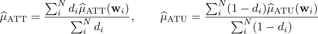
The treatment effects may be different between those who select the treatment and those who do not. Let w be a union of x and z: w = x ∪ z. ATT is the average effect of the treatment for those who actually select the treatment: µ _ATT(w) = E(y ₁ − y ₀ | x , d=1) = E(y ₁ − y ₀ | x , ν >− z ′γ). In contrast, ATU measures the average effect for those who do not receive the treatment: µ _ATU(w) = E(y ₁ − y ₀ | x , d = 0) = E(y ₁ − y ₀ | x , ν ≤ − z ′γ). The expectation conditional on the treatment status is

$E(y_j|x,d)=\text{exp}(x\prime {\beta }_j +{\sigma }_j^2/\text{2})\frac{\varphi \{(2d-1)({\rho }_j{\sigma }_j+{\text{z}}^{\prime }\gamma )\}}{\varphi \{(2d-1)({\text{z}}^{\prime }\gamma )\}}$

The unconditional versions of ATT and ATU are estimated by averaging over relevant subsamples:

${\widehat{\mu }}_{\text{ATT}}=\frac{{\displaystyle {\sum }_i^N{d}_i{\widehat{\mu }}_{\text{ATT}}({\text{w}}_i)}}{{\displaystyle {\sum }_i^N{d}_i}},{\widehat{\mu }}_{\text{ATU}}=\frac{{\displaystyle {\sum }_i^N(1-d_i){\widehat{\mu }}_{\text{ATU}}({\text{w}}_i)}}{{\displaystyle {\sum }_i^N(1-d_i)}}$

LATE is the average effect of the treatment for those who are induced to switch their treatment status in response to changes in an instrument variable. Suppose that a value of the kth variable of z, z_k changes from the lower value z_k,L to the upper value z_k,U . Accordingly, the treatment status changes; d = 0 with z _L′γ while d = 1 with z _U ′γ. Then, LATE can be defined as µ _LATE(w , z_k ) = E(y ₁ − y ₀ |x, − z _U ′γ ≤ ν ≤ − z _L′γ). The relevant conditional expectation of y_j is

$E(y_j|x,-{\text{z}}_U{\hspace{0.17em}}^{\prime }\gamma \le v\le -{\text{z}}_L{\hspace{0.17em}}^{\prime }\gamma )=\text{exp}(x\prime {\beta }_j +{\sigma }_j^2/\text{2})\frac{\varphi ({\rho }_j{\sigma }_j+{\text{z}}_L{\hspace{0.17em}}^{\prime }\gamma )}{\varphi ({\text{z}}_U{\hspace{0.17em}}^{\prime }\gamma )-\varphi ({\text{z}}_L{\hspace{0.17em}}^{\prime }\gamma )}$

Note that we cannot identify exactly which observations are induced to change the treatment status in response to the change in an instrument variable. Thus, it is standard to estimate the unconditional LATE as the average of the whole sample: ${\widehat{\mu }}_{\text{LATE}}(z_k)=N^{-}{\hspace{0.17em}}^{\text{1}}{\displaystyle {\sum }_{i=1}^N{\widehat{\mu }}_{\text{LATE}}(w_i,z_k)}$ . When there are multiple instrument variables, LATE can be defined for each instrument.

Finally, MTE measures the average effect of the treatment for those who have a particular value of ν. MTE at $\nu =\tilde{\nu }$ is ${\mu }_{\text{MTE}}(x,\tilde{\nu })=E(y_{\text{1}}-y_0|x,\nu =\tilde{\nu })$ . MTE evaluated at low values of $\tilde{\nu }$ measures the treatment effects for those less likely to receive the treatment, while MTE at high values of $\tilde{\nu }$ measures the treatment effects for those more likely to receive the treatment. The expected potential outcome conditional on $\nu =\tilde{\nu }$ is

$E(y_j|x,\nu =\tilde{\nu })=\text{exp{}x\prime {\beta }_j +{\rho }_j{\sigma }_j\tilde{\nu }+{\sigma }_j^2(\text{1}-{\rho }_j^2)/\text{2}}$

Like ATE and LATE, the unconditional version of MTE is estimated by averaging the whole sample: ${\widehat{\mu }}_{\text{MTE}}(\tilde{\nu })=N^{-}{\hspace{0.17em}}^{\text{1}}{\displaystyle {\sum }_{i=1}^N{\widehat{\mu }}_{\text{MTE}}(x_i,\tilde{\nu })}$ .

MTE is a unifying parameter in policy evaluation. ATE, ATT, and ATU can be expressed as weighted averages of MTE (Heckman and Vytlacil 2005). ATE is a simple average of MTE over the entire range of ν. ATT puts more weight on MTE at larger values of ν, that is, those more likely to select into the treatment. In contrast, ATU more heavily weighs those less likely to receive the treatment. MTE can also be interpreted as the limiting case of LATE as ${z^{\prime }}_U^{\hspace{0.17em}}\gamma \to z_L{\hspace{0.17em}}^{\prime }\gamma$ . Thus, it measures the ATE for those who are indifferent between receiving treatment and not at a given value of ν. By estimating MTE over a range of ν, we can understand how treatment effects are heterogeneous, and we can also tell who is more likely to benefit from marginal policy expansion. For example, constant MTE over ν indicates homogeneous treatment effects across different populations. Treatment effects can be heterogeneous. For example, MTE may be large among those unlikely to receive treatment. In this case, a policy maker may design an intervention targeting such a population to make the intervention more effective. Furthermore, MTE can be used to construct not only conventional treatment effects such as ATE and ATT but also treatment effects of hypothetical policy changes with different weights from ATE and ATT. See, for example, Heckman and Vytlacil (2005, 2007) for further discussion.

Note that the treatment-effect estimators in this article heavily rely on the assumption of joint normality discussed in section 2. Such parametric assumptions are often considered as restrictive in the recent literature of program evaluation, and the literature has moved toward less stringent assumptions in modeling and estimating causal effects. See, for example, Imbens and Wooldridge (2009). Indeed, several semiparametric estimators for MTE have been proposed. The package mtefe by Andresen (2018) implements several estimation methods for MTE. However, these estimators are not developed specifically for count-data outcome. Our treatment-effect estimators can serve as a benchmark estimation result in empirical studies with count-data outcome, although it is necessary to keep rather stringent distributional assumptions in mind.

As for the derivation of the asymptotic variance of these treatment-effect estimators, note that the estimation of the treatment effect involves two steps sequentially. The first step estimates the parameters of the switching regression model. Then, in the second step, the treatment effects are estimated using these estimated parameters. The asymptotic variance of the conditional treatment effects can be obtained by applying the delta method, which accounts for the fact that the parameters of the switching model are fit. To consistently estimate the asymptotic variances of the unconditional treatment effects, we must additionally consider the sampling variability from the randomness of w _i . Our derivation of the asymptotic variance is based on Newey and McFadden (1994). See also Terza (2016) for the correct asymptotic variance of sample means of nonlinear transformations such as our proposed treatment-effect estimators.

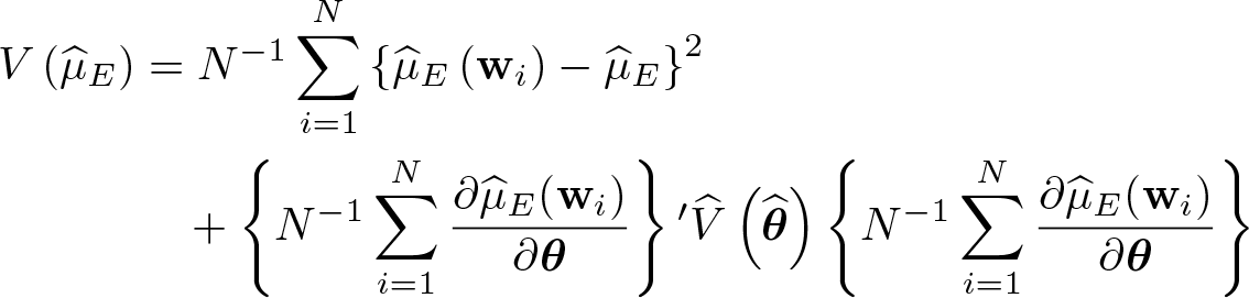
Assuming independence over observations, we estimate the asymptotic variance of the treatment-effect estimator by

$\begin{array}{l}V({\widehat{\mu }}_E)=N^{-1}{\displaystyle \sum _{i=1}^N{\{{\widehat{\mu }}_E({\text{w}}_i)-{\widehat{\mu }}_E\}}^2}\\ +{\left\{N^{-1}{\displaystyle \sum _{i=1}^N\frac{\partial {\widehat{\mu }}_E({\text{w}}_i)}{\partial \theta }}\right\}}^{\prime }\widehat{V}(\widehat{\theta })\left\{N^{-1}{\displaystyle \sum _{i=1}^N\frac{\partial {\widehat{\mu }}_E({\text{w}}_i)}{\partial \theta }}\right\}\end{array}$

where $\widehat{V}(\widehat{\theta })$ is the estimated asymptotic variance of $\widehat{\theta }$ for E = ATE, LATE, and MTE. The expressions for ATT and ATU are slightly different because we average over subsamples, but the essential structure is the same. The second term of this expression corresponds to the delta-method approach, and the first term reflects the variability arising from the randomness of w _i . Furthermore, one can estimate a cluster–robust variance estimator. The first term of the expression above becomes $N^{-1}{\displaystyle {\sum }_{g=1}^G{\left[{\displaystyle {\sum }_{g=1}^{N_g}\{{\widehat{\mu }}_E({\text{w}}_i)-{\widehat{\mu }}_E\}}\right]}^2}$ , where G denotes the number of clusters and N_g is the number of observations with each cluster such that $N={\displaystyle {\sum }_{g=1}^G{N}_g}$ . $\widehat{V}(\widehat{\theta })$ is replaced with the cluster–robust variance of θ in the second term.

4 The commands

This section describes the commands escount and lncount to implement the MLE of the models with lognormal latent heterogeneity. These commands use the Stata command ml, and likelihood-evaluator programs are written in Mata. We also describe the command teescount, which estimates the treatment effects after the execution of escount.

4.1 escount

Syntax

The syntax for the command is as follows:

escount depvar [=] indepvars [if] [in] [weight] [, select( depvar_s = varlist_s , noconstant offset( varname_o ) ) model( model ) noconstant exposure( varname_e ) offset( varname_o ) constraints( constraints ) intpoints( # ) vce( vcetype ) maximize_options]

aweights, fweights, iweights, and pweights can be used depending on the methods chosen; see [U] 11.1.6 weight.

Options

select( depvar_s = varlist_s , noconstant offset( varname_o ) ) specifies the variables and options for the selection equation. select() is required.

model( model ) specifies the distribution for count-data outcomes. The default is model(poisson). The alternative specification is nb.

noconstant suppresses a constant term of the outcome equation.

exposure( varname_e ) includes ln(varname_e ) in the model with the coefficient constrained to 1.

offset( varname_o ) includes varname_o in the model with the coefficient constrained to 1.

constraints( constraints ); see [R] Estimation options.

intpoints( # ) specifies the number of integration points to use for integration by quadrature. The default is intpoints(24); the maximum is intpoints(512).

vce( vcetype ) specifies the type of standard error reported, which includes types that are robust to some kinds of misspecification (robust), that allow for intragroup correlation (cluster clustvar), and that are derived from asymptotic theory (oim, opg); see [R] vce_option.

maximize_options: difficult, technique( algorithm_spec ), iterate( # ), [no] log, trace, gradient, showstep, hessian, showtolerance, tolerance( # ), ltolerance( # ), nrtolerance( # ), nonrtolerance, and from( init_specs ); see [R] Maximize. These options are seldom used.

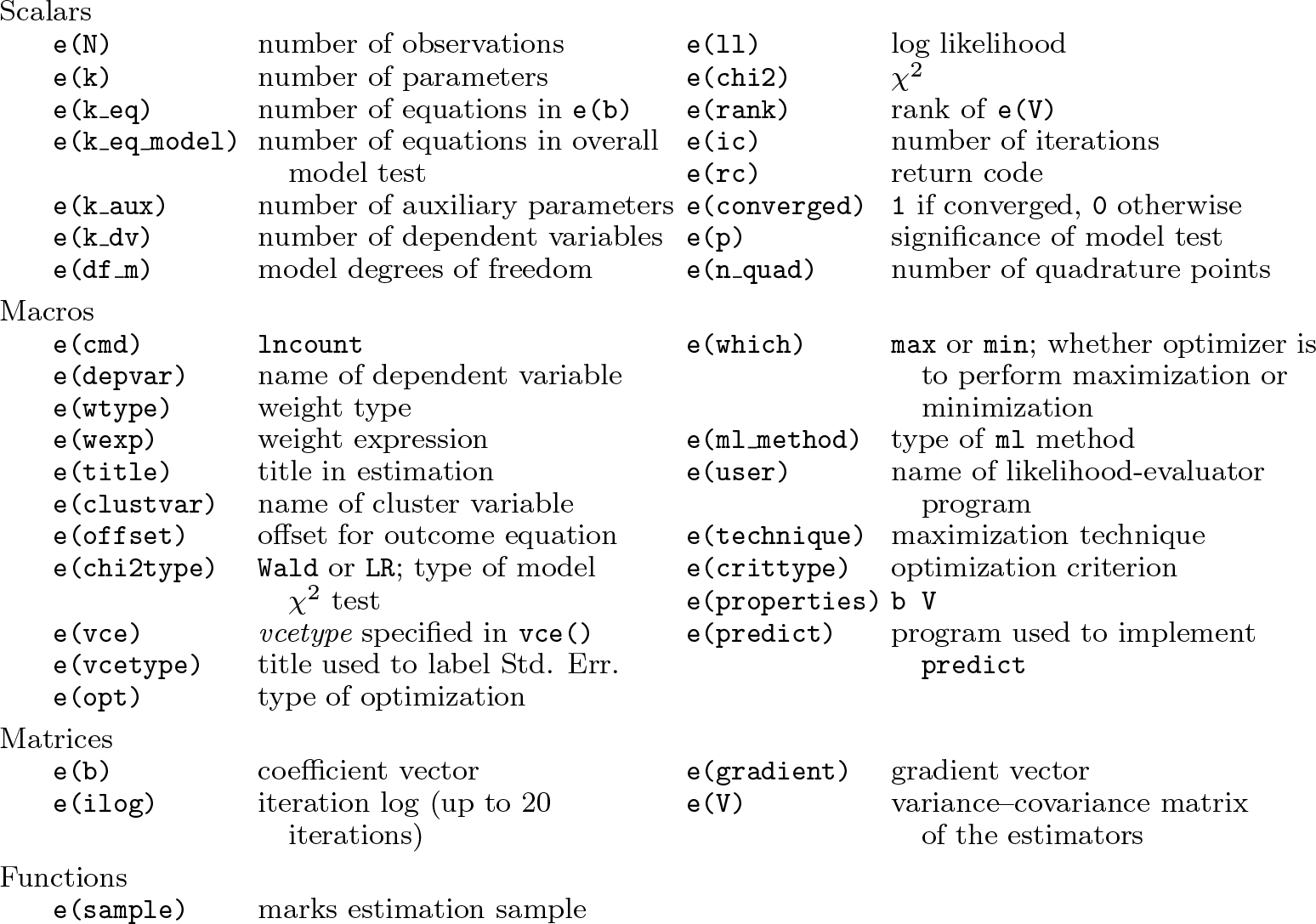
Stored results

escount stores the following in e():

Prediction

After an execution of escount, the predict command is available to compute several statistics with the following syntax:

predict [ type ] newvar [ if ] [ in ] [, psel xb0 xb1 xbsel mu0 mu1 mu0d0 mu0d1 mu1d0 mu1d1 ]

The options for predict are the following:

psel, the default, calculates the probability of receiving the treatment status d = 1 for each observation: Φ(z _i′γ).

xb0 calculates the linear prediction of the outcome variable of the treatment status d = 0 for each observation: x _i′β0.

xb1 calculates the linear prediction of the outcome variable of the treatment status d = 1 for each observation: x _i′β1.

xbsel calculates the linear prediction of the selection equation for each observation: z _i′γ.

mu0 calculates the expected value of the potential-outcome variable of the treatment status d = 0 for each observation: $E(y_0|x_i)=\text{exp}(x_i\prime {\beta }_0 +{\sigma }_0^2/\text{2})$ .

mu1 calculates the expected value of the potential-outcome variable of the treatment status d = 1 for each observation: $E(y_1|x_i)=\text{exp}(x_i\prime {\beta }_1 +{\sigma }_1^2/\text{2})$ .

mu0d0 calculates the expected value of the potential-outcome variable of the treatment status d = 0 conditional on receiving the treatment status d = 0 for each observation: $E(y_0|x_i,d=0)=\text{exp}(x_i\prime {\beta }_0 +{\sigma }_0^2/\text{2})\{\Phi (-{\rho }_0{\sigma }_0-z\prime \gamma )/\Phi (-z\prime \gamma )\}$ .

mu0d1 calculates the expected value of the potential-outcome variable of the treatment status d = 0 conditional on receiving the treatment status d = 1 for each observation: $E(y_0|x_i,d=\text{1})=\text{exp}(x_i\prime {\beta }_0 +{\sigma }_0^2/\text{2})\{\Phi ({\rho }_0{\sigma }_0+z\prime \gamma )/\Phi (z\prime \gamma )\}$ .

mu1d0 calculates the expected value of the potential-outcome variable of the treatment status d = 1 conditional on receiving the treatment status d = 0 for each observation: $E(y_{\text{1}}|x_i,d=0)=\text{exp}(x_i\prime {\beta }_{\text{1}} +{\sigma }_1^2/\text{2})\{\Phi (-{\rho }_{\text{1}}{\sigma }_{\text{1}}-z\prime \gamma )/\Phi (-z\prime \gamma )\}$ .

mu1d1 calculates the expected value of the potential-outcome variable of the treatment status d = 1 conditional on receiving the treatment status d = 1 for each observation: $E(y_{\text{1}}|x_i,d=\text{1})=\text{exp}(x_i\prime {\beta }_{\text{1}} +{\sigma }_1^2/\text{2})\{\Phi ({\rho }_{\text{1}}{\sigma }_{\text{1}}+z\prime \gamma )/\Phi (z\prime \gamma )\}$ .

4.2 teescount

Syntax

The syntax for the command is as follows:

teescount [, ate att atu late( varname lower upper ) mte( nu )]

This command estimates the treatment effects and their standard errors using the estimated parameters of the switching regression model with count-data outcomes. It can be executed only after the execution of escount.

Options

ate estimates ATE. This is the default.

att estimates ATT.

atu estimates ATU.

late( varname lower upper ) estimates LATE when the value of varname (z_k ) changes from lower (z_k,L ) to upper (z_k,U ). lower and upper should be numerical.

mte( nu ) estimates MTE evaluated at nu (ν). nu should be numerical.

Stored results

teescount stores the following in r():

Matrices

The matrix r(table) contains the estimated treatment effect in the first column, its standard error in the second column, the z-value in the third column, and the p-value in the fourth column. When only one option is specified, this matrix is a row vector. When more than one option is specified, the rows of this matrix correspond to the treatment effects that are specified as options.

4.3 lncount

Syntax

The syntax for the command is as follows:

lncount depvar [= ] indepvars [if] [in] [weight] [, model( model ) noconstant exposure( varname_e ) offset( varname_o ) constraints( constraints ) intpoints( # ) vce( vcetype ) maximize_options]

aweights, fweights, iweights, and pweights can be used depending on the methods chosen; see [U] 11.1.6 weight.

Options

model( model ) specifies the distribution for count-data outcomes. The default is model(poisson). The alternative specification is nb.

noconstant suppresses a constant term of the outcome equation.

exposure( varname_e ) includes ln(varname_e ) in the model with the coefficient constrained to 1.

offset( varname_o ) includes varname_o in the model with the coefficient constrained to 1.

constraints( constraints ); see [R] Estimation options.

intpoints( # ) specifies the number of integration points to use for integration by quadrature. The default is intpoints(24); the maximum is intpoints(512).

vce( vcetype ) specifies the type of standard error reported, which includes types that are robust to some kinds of misspecification (robust), that allow for intragroup correlation (cluster clustvar), and that are derived from asymptotic theory (oim, opg); see [R] vce_option.

maximize_options: difficult, technique( algorithm_spec ), iterate( # ), no log, trace, gradient, showstep, hessian, showtolerance, tolerance( # ), ltolerance( # ), nrtolerance( # ), nonrtolerance, and from( init_specs ); see [R] Maximize. These options are seldom used.

Stored results

lncount stores the following in e():

Prediction

After an execution of lncount, the predict command is available to compute several statistics with the following syntax:

predict [ type ] newvar [ if ] [ in ] [, n xb ]

The options for predict are the following:

n computes the predicted number of events for each observation: exp(x _i′β+σ ² /2). This is the default.

xb computes the linear prediction of the dependent variable for each observation: x _i′β.

4.4 Notes

In the MLE, σ and ρ are not directly estimated to guarantee that σ > 0 and −1 < ρ < 1. Instead, ancillary parameters ln σ and ρ^∗ are estimated. These ancillary parameters are transformed as σ_j = exp(ln σ_j ) and ρ_j = {exp(ρj^∗ ) − exp(−ρj^∗ )}/{exp(ρj^∗ ) + exp(−ρj^∗ )}. The estimates of these ancillary parameters are respectively reported as lnsigma and athrho, while the estimates of these transformed parameters are reported as sigma and rho. For the switching model, the estimates of the ancillary and transformed parameters are reported with 0 or 1 indicating the treatment status. Similarly, when model is nb, the ancillary parameter ln α is estimated and then transformed to α. The estimates of these parameters are reported as lnalpha and alpha, respectively.

5 Example

To illustrate the use of escount, we show some examples using a dataset from the Stata website. This is the same dataset used for the example of etpoisson and a simulated random sample of households. The outcome of interest is the number of trips (trips), and a possible endogenous treatment indicator is car ownership (owncar). There are some other controlling variables of household characteristics. realinc, which is the ratio of household income to the median income of the census tract, serves as an instrumental variable. See the example in [TE] etpoisson for the details.

First, we execute escount to fit the switching regression model with the Poisson specification. It is followed by the command that tests whether the self-selection matters, that is, tests the null hypothesis H ₀ : ρ ₀ = ρ ₁ = 0. It is equivalent to testing H ₀ : ρ0 ^∗ = ρ1 ^∗ = 0. ¹

This is the result of MLE of the switching regression model with count-data outcomes. Each of the coefficients of correlation between ν and ε_j for j = 0, 1 is statistically significant at any meaningful level. The result of the test command also shows that these parameters are jointly significant. These results indicate the presence of the self-selection problem. Households that tend to own a car are more likely to make a trip, even controlling for observable characteristics. Without considering the self-selection, the estimation of the treatment effects is biased.

Next, we estimate the treatment effects: ATE, ATT, and ATU. We also report the estimated LATE when the value of realinc changes from 1.0 to 1.1, which may not necessarily be an interesting quantity but is shown for illustration. Besides, we also show the estimated treatment effects ignoring the self-selection problem, that is, restricting ρ ₀ = ρ ₁ = 0.

The estimated treatment effects from the model without considering the self-selection problem are more than twice as large as those from the switching regression model. This result is consistent with the positive values of the estimated ρ ₀ and ρ ₁. Ignoring the self-selection problem results in the upward biases of the treatment effects. Note that when ρ ₀ = 0 and ρ ₁ = 0, the treatment effects are not heterogeneous so that ATE and LATE are the same. Although not reported here, MTE is also constant at the same value as ATE and LATE over the entire range of ν. The reason why ATT and ATU are different is that we average over different subsamples to obtain the unconditional effects.

When considering the self-selection issue, we find that ATE is marginally significant at the 5% level. Although ATU is highly significant, ATT is not significant even at the 10% level. The insignificance of ATT may be due to the efficiency loss from the estimation of the switching regression model. An endogenous dummy variable model may be parsimonious and lead to a more efficient estimator when the restrictions that σ ₀ = σ ₁, ρ ₀ = ρ ₁, and β0 = β1, except for constant terms being correct. As shown below, when we conduct the Wald test of the restrictions, we fail to reject the null hypothesis with the p-value of 0.3472.

Given this result, we next fit the model and the treatment effects under the restrictions. For comparison and as an example of lncount, we also fit the dummy variable model without considering the self-selection issue.

The estimation result of the restricted model, that is, the endogenous dummy variable model, is identical to the result from the built-in command etpoisson, which is not reported here. The coefficient on the endogenous dummy variable corresponds to the difference in the constant terms between the treatment statuses. The command lincom returns the estimated difference. This estimate is much lower than the estimated coefficient on owncar from lncount, which ignores the endogeneity of car ownership. The estimates of the treatment effects based on the endogenous dummy variable model are similar to those from the switching regression model, but with smaller standard errors.

Based on the endogenous dummy variable model, we estimate and plot MTEs over normalized values of ν with 95% confidence intervals. The normalized value of ν is Φ(ν), and thus it takes values between 0 and 1. It represents the propensity for treatment. MTE and its standard error are estimated at each point of the normalized value using a loop.

Figure 1 presents the estimated MTEs. The figure shows that MTE increases with higher propensity for treatment. The effect of car ownership on the number of trips is larger for a household that is more likely to own a car. The result, that ATT is larger than ATU, reflects this upward slope of MTE. At higher values of treatment propensity, where ATT puts more weight on MTE, the treatment effect is larger.

Figure 1.

MTEs

6 Conclusion

In estimating the effects of treatment, endogeneity is a common problem that researchers face. Researchers in health economics and other applied microeconomics also come across count-data outcomes frequently. It is important to equip researchers with a statistical tool to address endogenous treatment with a count-data outcome. In this article, I introduced the command escount, which implements the MLE of the endogenously switching regression model with count-data outcomes, where a possible outcome differs between different treatment statuses and an individual selects into one of the statuses endogenously. Based on lognormal latent heterogeneity, the model allows for the dependence between the selection process and potential outcomes. After one estimates the parameters of the switching regression model, various treatment effects can be estimated with the command teescount.

Supplemental Material

Supplemental Material, st0612 - Endogenous switching regression model and treatment effects of count-data outcome

Supplemental Material, st0612 for Endogenous switching regression model and treatment effects of count-data outcome by Takuya Hasebe in The Stata Journal