Comparing distributions of ordinal data

Abstract

To compare distributions of ordinal data such as individuals’ responses on Likert-type scale variables summarizing subjective well-being, we should not apply the toolbox of methods developed for cardinal variables such as income. Instead, we should use an analogous toolbox that accounts for the ordinal nature of the responses. In this article, I review these methods and introduce a new command, ineqord, for undertaking distributional comparisons. As the empirical illustrations demonstrate, ineqord can be used for dominance checks as well as for estimation of indices of polarization and inequality.

1 Introduction

This article is about how to compare distributions of personal well-being where wellbeing is measured using an ordinal scale, and it introduces a new command, ineqord, for undertaking these comparisons.

Leading examples of personal well-being indicators are self-assessed (“subjective”) life satisfaction or health status for which individuals provide responses on a Likert-type scale. For instance, regarding life satisfaction, respondents may be presented with a linear integer scale running from 0 to 10 (11 levels) and asked to respond to the question “Overall, how satisfied are you with your life nowadays where 0 is ‘not at all satisfied’ and 10 is ‘completely satisfied’?” (Data based on this scale are used in section 4.) Other life satisfaction scales use 5, 7, or 10 levels. Some subjective well-being (SWB) scales employ a mixture of negative and nonnegative integers to label the levels. For example, people are asked to rate how satisfied they are with their life, choosing between “completely dissatisfied” (scaled as −3), “mostly dissatisfied” (−2), “somewhat dissatisfied” (−1), “neither satisfied nor dissatisfied” (0), “somewhat satisfied” (1), “mostly satisfied” (2), and “completely satisfied” (3).

SWB measures are increasingly being used in tandem with the monetary measures of personal economic well-being such as income or wealth that national and international statistical agencies and most researchers have conventionally focused on. A catalyst for the new emphasis was the “Report by the Commission on the Measurement of Economic Performance and Social Progress” (Stiglitz, Sen, and Fitoussi 2009), which set out a comprehensive agenda for going “Beyond GDP”. The report’s Quality of Life sections emphasize that “well-being is multidimensional” (2009, 14) and that “objective and subjective dimensions of well-being are both important” (2009, 16). The Organisation for Economic Co-operation and Development (OECD) has played an important role in implementing the report’s recommendations in this area, launching its Better Life Initiative (in 2011), regularly reporting on well-being outcomes (How’s Life; see, for example, OECD [2020]), and developing the Better Life Index and multiple online resources (see https://www.oecd.org/statistics/better-life-initiative.htm). In parallel, the national statistical agencies of OECD member countries have introduced initiatives to address the Beyond GDP agenda, including a greater emphasis on collection of and reporting on SWB data.

Income and wealth are cardinal variables, and there are well-established methods for comparing distributions of them in terms of levels and inequality. There are also many community-contributed commands for undertaking distributional comparisons of cardinal variables, including my ineqdeco, ineqdec0, sumdist, and svylorenz, svyatk and svygei (with Martin Biewen), and glcurve (with Philippe Van Kerm), all available from the Statistical Software Components (SSC) archive.

In contrast, SWB measures are ordinal in nature, which raises the question of how to undertake distributional comparisons in this situation. How do we assess whether average well-being or well-being inequality has increased over time or differs between countries or social groups? A growing literature (cited below) has shown on the one hand that it is inappropriate to apply comparison methods developed for cardinal well-being measures to ordinal SWB measures, although many researchers continue to do this—the World Happiness Report (Helliwell, Huang, and Wang 2019) is a leading example. However, on the other hand, there is now a toolbox of methods for application to ordinal data that is analogous to the toolbox long applied to distributions of cardinal variables such as income. See Jenkins (Forthcoming) for development of this argument and illustrations. ineqord provides the means to implement methods that are appropriate for comparisons of distributions of ordinal data.

ineqord produces estimates of inequality and polarization indices: the Allison–Foster index, the normalized average jump index, multiple Apouey indices, multiple Abul Naga–Yalcin indices, multiple Cowell–Flachaire indices, and Jenkins indices. Optionally, ineqord also derives estimates of cumulative distribution functions (CDFs) and related objects that can be used to describe ordinal distributions and to undertake dominance checks of differences between distributions.

ineqord assumes the user has respondent-level data with responses referring to ordinal well-being scores. If the user has grouped data describing the distribution of the well-being variable, the user needs first to construct a dataset using this information. See section 4 for illustrations.

2 Comparisons of distributions of ordinal data

This section provides a brief overview of methods used for undertaking comparisons of distributions of ordinal data and discusses ineqord‘s functionality against this background.

Let us suppose that we have individual-level SWB data held in a variable called swb. The inequality and polarization indices calculated by ineqord summarize dispersion in the distribution of responses across the levels of swb. There are K ≥ 3 levels of the ordinal variable in principle, though one or more levels might receive no responses in practice, a situation to which I return below. The levels have numerical labels c ₁ , c ₂ ,…, c_K , where −∞ < c ₁ < c ₂ < · · · < c_K < ∞. The “linear integer” scale is the one with c_k = k, for each k = 1, 2,…, K. The empirical distribution of responses is described by the proportion of the individuals who report the kth level, f_k , for each k. The CDF is described by the proportion of individuals reporting the kth level or lower, $F_k={\displaystyle \sum { }_{j=1}^k} f_k$ , for each k. The survivor function is described by the proportion of individuals reporting the kth level or higher, $S_k={\displaystyle \sum { }_{j=k}^k}{j}_k$ , for each k. This is a nonstandard definition—usually the survivor function is defined as 1 − F_k —but it is what is used to characterize a class of Cowell–Flachaire inequality indices (see section 2.2).

A commonly used measure of inequality of such ordinal data, especially life satisfaction and happiness data, is the standard deviation. Use of this measure is inappropriate because it assumes that swb is measured on a ratio scale. Kalmijn and Veenhoven (2005) acknowledge this issue but claim that the standard deviation is an appropriate measure nonetheless.

Economists specializing in inequality measurement have long been critical of the application to ordinal data of the standard deviation and other inequality indices typically applied to variables measured on a ratio scale. These indices use the mean as the reference point for assessing spread, but with ordinal data, the value of the mean is contingent on the scale used. Orderings of distributions according to their means or standard deviations are not robust to changes in the scale used.

Critiques by economists include the papers by Allison and Foster (2004), Cowell and Flachaire (2017), and Dutta and Foster (2013). These authors and others propose measures that respect the ordinal nature of the data. In one tradition, indices characterize greater inequality as greater spread about the median. The other tradition characterizes greater inequality as greater spread away from a maximum value.

2.1 Polarization indices

The Allison–Foster index is the difference between the mean score for respondents with scores above the median minus the mean score for respondents with scores below the median. This index was first proposed by Allison and Foster (2004). Dutta and Foster (2013) provide more extensive discussion of it, and the formulas used by ineqord are based on their equations 1 and 2 (page 398).

The two-parameter indices proposed by Abul Naga and Yalcin (2008), ANY(a, b), with a, b ≥ 1, are a form of weighted difference between the cumulative percentages of individuals in the lower half of the distribution and the cumulative percentages in the upper half of the distribution. The parameters tune the weights given to the two halves. ANY(1, 1) weights the two halves equally. Broadly speaking, when b > a, ANY(a, b) gives greater weight to the bottom half of the distribution; when a > b, it gives greater weight to the top half of the distribution. According to Abul Naga and Yalcin (2008, 1621), “For a given value of β,…, as α → ∞, the inequality index abstracts from the dispersion below the median.” (Their α and β correspond to my a and b.) On the other hand, when b > a, ANY(a, b) gives greater weight to the bottom half of the distribution. For a given value of a, choosing larger values of b places less weight on the distribution in categories above the median. In the limiting case when b → ∞, only below-median categories are relevant. Thus, for example, the indices ANY(1, 1), ANY(1, 2), and ANY(1, 4) give increasingly greater weight to the lower half of the distribution when assessing overall polarization.

Apouey’s (2007) P 2(e) indices each aggregate the “distances” between F_k and 0.5 (the value of F_k at the median) across the levels of swb. P 2(0.5) uses the square root of the absolute differences to summarize distance, and P2(1) uses a “city block” (linear) distance function. P 2(2) uses a Euclidean distance metric and is the same as the 1−l ² index of Blair and Lacy (2000). (The Blair–Lacy index may also be calculated using Lacy’s (2010) community-contributed ordvar command, available from the SSC archive.) In general, the value of parameter e determines how concentration within the groups below the median and within the groups above the median contributes to overall polarization.

The average jump index is the average across respondents of the absolute difference between each observed value of swb and the median value, normalized by the maximum value for the index. For a linear integer scale, the average jump index equals the Allison–Foster index divided by the total number of levels of swb minus one (Allison and Foster 2004, 514). In this case, the index summarizes the (normalized) average number of category “jumps” required to change from the observed level to the median level. For a linear integer scale, the average jump index is the same as the ANY(1, 1) index and the P2(1) index.

2.2 Inequality indices

Cowell and Flachaire (2017) build inequality measures from axiomatic first principles, providing two families of one-parameter indices based on downward-looking and upwardlooking measures of individual “status”, respectively. ineqord uses the “peer-inclusive” (rather than “peer-exclusive”) definitions of these, reflecting the focus of Cowell and Flachaire (2017) and other authors. For an individual reporting a response corresponding to the kth level of the scale, peer-inclusive downward-looking status is given by F_k , and peer-inclusive upward-looking status is given by S_k . The inequality indices aggregate “distances” between each individual’s status and the maximum possible status value (which is one, given his or her definition of status).

Members of the two Cowell–Flachaire inequality index families I(α) are distinguished by parameter α, which encapsulates the sensitivity of overall inequality to the dispersion of individual status in different ranges of the status distribution, with 0 ≤ α < 1. The smaller that α is, the more sensitive is the overall index to differences in status at the bottom of the status distribution rather than at the top. If the distribution of responses on swb is symmetric across the levels, F_k = S_k , and each downward-looking Cowell–Flachaire index has the same value as its upward-looking counterpart with the same α.

Jenkins’s (2019) J_d index is defined for Cowell–Flachaire’s peer-inclusive downwardlooking status measure, and his J_u index is defined for their peer-inclusive upwardlooking status measure. Each index is equal to the area between the generalized Lorenz (GL) curve for the relevant status distribution and the GL curve for the distribution with no status inequality [in which case the GL curve is a straight line between the origin and point (1, 1)], divided by the total area beneath the perfect equality curve (= 0.5). Equivalently, each index is equal to one minus twice the area beneath the GL curve for status. The GL curve for status, GL(p), plots cumulative status per capita against cumulative population share, 0 ≤ p ≤ 1, of individuals ranked in ascending order of status. GL(0) = 0 and GL(1) is the arithmetic mean of status. See Jenkins (2019) for details.

2.3 Index properties

All the polarization and inequality indices calculated by ineqord equal their minimum value, zero, if all respondents report the same value for swb. The Allison–Foster, average jump, Apouey, and Abul Naga–Yalcin indices each summarize polarization of responses relative to the median. These indices reach their maximum value when half the responses on swb refer to the minimum value of the scale and half the responses refer to the maximum value; that is, the distribution of responses is totally polarized. In this case, the maximum value equals one—except for the Allison–Foster index, for which the maximum value depends on the number of categories.

Cowell–Flachaire I(α) and J indices need not reach a maximum value with this distribution of responses: this is because the indices summarize inequality as spread rather than as polarization. For example, for any given K, I(α) and J indices record greater inequality for a uniform distribution than for a totally polarized distribution (Jenkins 2019).

I(α) and J indices are invariant to order-preserving transformations of the ordinal scale variable, that is, scale independent. The Allison–Foster index is not scale independent, and hence, Dutta and Foster (2013), in their empirical application, provide estimates based on linear, convex, and concave scales. Abul Naga–Yalcin and Apouey indices are scale independent (but also see the remarks in section 2.5).

2.4 Dominance checks for unanimous orderings by classes of indices

ineqord also provides users with the ability to undertake dominance checks. In general, dominance means that finding an appropriately defined graph for one distribution lies everywhere on or above the corresponding graph for another distribution is equivalent to a unanimous ranking of the two distributions by all measures satisfying a specific set of properties. There are several different types of dominance in this context.

Allison and Foster (2004) provide results for “F-dominance” and “S-dominance”. The former refers to comparisons of CDFs and rankings by average well-being levels (first-order dominance): if the CDF for distribution A lies everywhere on or above the CDF below that for distribution B, then A has higher average well-being than B, regardless of scale. S-dominance (spread dominance) refers to comparisons of S-curves, which are derived from CDFs, so the criterion can also be expressed in terms of these. That is, if A and B have the same median, and the CDF for A lies above that for B at scale values below the median but above that for B at scale values at the median and above, all polarization indices respecting the property that greater spread about the median corresponds to greater polarization will show A as having greater polarization than B. S-dominance can arise only if the pair of distributions have a common median and if there is no F-dominance.

Jenkins (2019) shows that, for each of the two Cowell–Flachaire definitions of status, if the GL curve for status distribution A lies nowhere above the GL curve for status distribution B, all Cowell–Flachaire I(α) indices and the J index will record A as having more inequality than B. These GL curve comparisons can be applied if the distributions have different medians.

ineqord can also be used to undertake the H-dominance checks proposed by Gravel, Magdalou, and Moyes (Forthcoming). These authors start from the principle that the inequality of an ordinal variable increases if there is a shift in density mass away from a specific level (one person moving up a level and one moving down). This is the concept of a disequalizing “Hammond transfer” (compare the concept of a disequalizing Pigou–Dalton transfer for a cardinal variable such as income). Gravel, Magdalou, and Moyes (Forthcoming) define H ⁺ and H⁻ curves (called H and $\overline{H}$ curves in their article), which are specifically defined recursive cumulations of CDFs (just as GL curves are but differently defined). The authors prove a dual dominance result: distribution A being more equal than distribution B according to the Hammond transfer concept is equivalent to finding (i) the H ⁺ curve for A lying nowhere above the H ⁺ curve for B and (ii) the H⁻ curve for A lying nowhere above the H⁻ curve for B. They also show that, if there is F -dominance, there is also H ⁺ dominance. The dual dominance check can be applied if the distributions have different medians.

Gravel, Magdalou, and Moyes (Forthcoming) do not refer to any existing indices when discussing their dual dominance criteria. The relationships between the dual dominance and GL dominance criteria are a topic of current research.

2.5 Some computational and conceptual issues

For correct calculation of the Abul Naga–Yalcin, average jump, Apouey, and Jenkins indices, ineqord must know the total number of possible levels of the ordinal response variable. This number may be greater than the maximum observed in the data, for example, if there are no responses on some scale values or if there is total polarization. By default, ineqord assumes that the total number of possible levels of the ordinal response is the number of levels observed containing responses. If this assumption is incorrect, it is the user’s responsibility to specify the maximum number of levels of response using the nlevels() option, described below. See also the discussion of scale dependence below.

Apouey P2(e) indices refer to the case in which the ordered-response categories are labeled with positive integers (1 for the lowest level, 2 for the second-lowest level, etc.), which is a linear integer scale. For correct calculation of these indices, it is the user’s responsibility to check that the scale underlying swb is appropriate. Optionally, ineqord relabels the observed responses to calculate the Apouey indices using a linear transformation: response new = response − minlevel + 1, where minlevel is the value specified by the minlevel() option and response in this case would be swb. For example, with the option, the life satisfaction scale cited above (0, 1,…, 10) is converted to (1, 2,…, 11) by setting minlevel = 0. Scale (−1, 0, 1) is converted to (1, 2, 3) by setting minlevel = −1. Be aware that if the response scale values were instead (2, 4, 6), say, and the user sets minlevel = 2, ineqord‘s calculation would be based on transformed responses (1, 3, 5), not (1, 2, 3), and correct calculation of the Apouey (and J) indices would also require setting the maximum number of levels to 5 using the nlevels() option. Calculation of the indices would assume that scale values 2 and 4 are possible (and this is relevant to the assessment of how polarized swb is), but there are no responses observed for them. On related issues, see the discussion of the “mergers principle” by Cowell and Flachaire (2017).

The precise definition of the median is fundamental to the estimation of polarization indices. I use Stata’s definition of the median, as set out in Methods and formula of [R] summarize, with one rarely used modification.

There are other possible definitions of the median. For example, Abul Naga and Yalcin’s definition is that level “m is the median…if P_{m− 1} ≤ 0.5 and P_m ≥ 0.5” (2008, 1616), where P_k is the fraction of individuals reporting level k or less, that is, what I have referred to as F_k . The definition means that the median is undefined if the fraction reporting the lowest level k = 1 is greater than one half (P ₁ > 0.5), though, of course, this case is likely to be rare in practice. Cowell and Flachaire (2017, 300) discuss other potential issues and refer to them when motivating their nonmedian-based approach.

Although use of Stata’s definition of the median almost invariably works well in real-world situations, there is one tricky special case to deal with—the situation in which Stata reports a noninteger median (having taken the average value of the scale in two adjacent categories—see the Stata Base Reference Manual again). This is most likely to occur if there are scale levels in the middle of the range that do not receive any responses. Using a noninteger median “as is” leads to an error when calculating ANY indices using Abul Naga and Yalcin’s (2008) formulas. Thus, the code for ineqord uses Stata’s definition by default except that, in the (rarely experienced) noninteger median case, it applies the ceil() function to the noninteger median and then proceeds using the revised (integer-valued) median. If ceil() changes the median, r(newmedian) differs from r(median) in the stored results. With this adjustment, ineqord generates the estimates expected.

Bootstrapped standard errors for the indices can be derived using bootstrap or, for example, rhsbsample (Van Kerm 2013) implementing Saigo, Shao, and Sitter’s (2001) repeated half-sample bootstrap approach. See section 4 below. Analytical formulas for variance estimates exist for some of the indices and curve ordinates but not for all of them, and the formulas that are provided do not account for sample design features such as weights, clustering, or stratification.

Finally, note that the indices and the dominance results cited earlier refer to levels and dispersion of a categorical well-being variable with an arbitrary scale. They do not refer to levels and dispersion of some underlying unobserved SWB variable. This is an important distinction because it is often assumed that discrete categorical responses on a Likert-type scale are manifestations of a latent continuous variable. For example, Delhey and Kohler’s (2011) adjustment to the standard deviation measure to account for the bounded nature of a Likert-type scale, implemented in sdlim on the SSC archive, refers to a latent SWB variable. Stevenson and Wolfers (2008) suppose that the ordinal data responses are realizations of a latent continuous well-being variable that is assumed to be normally distributed within a population, with moments of the latent variable estimated using ordinal regression techniques. Bond and Lang (2019) emphasize the distinction between manifest categorical and latent continuous SWB variables, and they highlight the strong assumptions required to identify distributions of the latter from the former. More positively, Kaplan and Zhuo (2019) provide some results about what can be learnt about latent SWB distributions when manifest categorical distributions are available.

3 The ineqord command

3.1 Syntax

This section describes the syntax of the ineqord command. The command works with Stata 14 or later.

ineqord varname [if] [in] [weight] [, alpha(#) nlevels(#) minlevel(#) ustatusvar(string) dstatusvar(string) catvals(string) catprops(string) catcprops(string) catsprops(string) gldvar(string) gluvar(string) hplus(string) hminus(string) ]

by and statsby are allowed; see [U] 11.1.10 Prefix commands.

aweights, fweights, iweights, and pweights are allowed; see [U] 11.1.6 weight.

3.2 Options

alpha( # ) calculates an additional Cowell–Flachaire index with parameter value α. The value must be between 0 and 1.

nlevels( # ) specifies the total number of possible levels of the ordinal response variable. nlevels() is required for correct calculation of the Blair–Lacy and Apouey indices if the observed number of levels is less than the maximum possible.

minlevel( # ) specifies the minimum level of the ordinal response variable. minlevel() is required for correct calculation of the Blair–Lacy and Apouey indices if the observed minimum is not equal to 1.

ustatusvar( string ) saves the Cowell–Flachaire upward-looking status variable after calculation.

dstatusvar( string ) saves the Cowell–Flachaire downward-looking status variable after calculation.

catvals( string ) saves the distinct values of the response variable after calculation. There is one value per level.

catprops( string ) saves the sample proportions for each level after calculation. catcprops( string ) saves the sample cumulative proportions after calculation. catsprops( string ) saves the sample cumulative survivor proportions after calculation.

gldvar( string ) saves the GL ordinates of the Cowell–Flachaire downward-looking status variable after calculation.

gluvar( string ) saves the GL ordinates of the Cowell–Flachaire upward-looking status variable after calculation.

hplus( string ) saves the ordinates of H ⁺ curve after calculation.

hminus( string ) saves the ordinates of H⁻ curve after calculation.

ustatusvar() and dstatusvar() are observation-level variables. cat * (), gl * (), and h * () are category-level variables (with K values). See section 4.

3.3 Stored results

ineqord stores the following in r():

4 Examples

This section illustrates ineqord in action. For further examples of distributional comparisons based on numerical indices and dominance checks applied to World Values Survey data on life satisfaction, see Jenkins (Forthcoming, 2019). These data were also used by Cowell and Flachaire (2017), and ineqord produces the same estimates that they report—they focus on I(0) using both peer-inclusive downward and upwardlooking definitions of status.

4.1 Life satisfaction data from the UK Annual Population Survey (APS)

Most of my examples are based on data about life satisfaction drawn from the Annual Population Survey (APS) Three-Year Pooled Dataset January 2015–December 2017 (Office for National Statistics, Social Survey Division 2018), a nationally representative survey of UK adults. The data and documentation are downloadable from the UK Data Service by researchers who register. For brevity, I refer to the data as “the APS”. Data drawn from the APS are used by the UK’s Office for National Statistics to provide annual reports on personal well-being; see, for example, Office for National Statistics (2019).

The dataset contains 530,300 (unweighted) observations of which 275,336 provide a nonmissing response to the life-satisfaction question set out in section 1. Responses are held in the variable named SATIS. Sample weights are provided in variable PWTA17C. Missing values are recorded as values of −8 and −9 and all variables names are in uppercase. Before any use of ineqord, I convert the missing values to Stata missing values and, for convenience, put all variable names in lowercase.

Only around 12% of respondents report a value of 5 or lower on the 0 to 10 scale. Almost 15% report that they are completely satisfied with their life (scale point 10), with the modal value equal to 8.

To proceed further, we have to address the fact that the linear integer scale runs from 0 to 10. It does not start at 1. If ineqord were applied ignoring this, it would provide incorrect estimates for some of the indices. There are two ways to proceed: either 1) create a new variable to ensure the scale goes from 1 to 11 and then run ineqord using this variable; or 2) run ineqord using its minlevel(0) option and the variable satis. To implement strategy 1, I create a new variable named ls:

Applying strategy 2, we derive the following estimates for the UK adult population. It is easily verified that the code ineqord ls [aw = pwta17c] gives exactly the same estimates as those shown, whereas ineqord satis [aw = pwta17c] gives incorrect estimates (output not shown).

The first components of the output provide descriptive statistics. For example, we see that the median response is 8 on the 0–10 scale. The average jump index estimate is 0.24514. Because we have a linear integer scale, the average number of category “jumps” required to change from the observed level to the median level (normalized by the total number of levels minus one = 10) is 0.24514 and is also equal to the estimates of ANY(1, 1) and P2(1) in this case. The Allison–Foster index value, 2.45139, is 10 times the average jump index.

The earlier tabulation of satis shows dispersion in life-satisfaction responses, and this is reflected in estimates of the indices of polarization and inequality that are greater than 0. The specific values of the estimates are otherwise hard to interpret; they become more valuable when there are estimates from multiple distributions that can be compared.

Let us therefore proceed to some distributional comparisons, considering how life satisfaction distributions differ between UK adults according to their marital status. I create a new variable, mstat, collapsing the information held in the marsta variable. I treat individuals in a cohabiting relationship as married.

A first look at the distributions of life satisfaction broken down by marital status indicates that married individuals are more satisfied than single, never married (SNM) or separated, divorced, or widowed (SDW) individuals. (In what follows, I ignore the “other” group given their small size.) For convenience, I use the rescaled variable ls henceforth (rather than satis).

4.2 Dominance checks

I begin by reporting dominance checks rather than indices, for two reasons. First, from a robustness point of view, it is useful to know whether a pair of distributions can be unanimously ranked by all indices of a given family sharing key common characteristics. Even if you and I disagree about which is the best index within the family but there is dominance, you and I will agree about how to rank a pair of distributions—though of course we may disagree about the magnitudes of differences. Second, because dominance checks are usually implemented using graphs, using them is also a way of “showing the data”.

All the raw materials for the various dominance checks can be created by ineqord using the cat * (), gl * (), and h * () options shown in the syntax diagram. When ineqord runs using these options, it creates new variables that can be listed or displayed graphically. To compare distributions of life satisfaction by marital status group, I run the following code. The output for the indices is not shown here but is summarized later.

A listing of the values of new variables for married individuals is shown below. Going from left to right, we see there are scale labels followed by the estimates of the density function, the CDF (with estimates corresponding to those shown by the earlier tabulate command), the survivor function, GL ordinates for (peer-inclusive) downward-looking status, and H ⁺ and H⁻ ordinates, respectively. ineqord creates the zeros in the bottom row by default to facilitate drawing of GL and H curves.

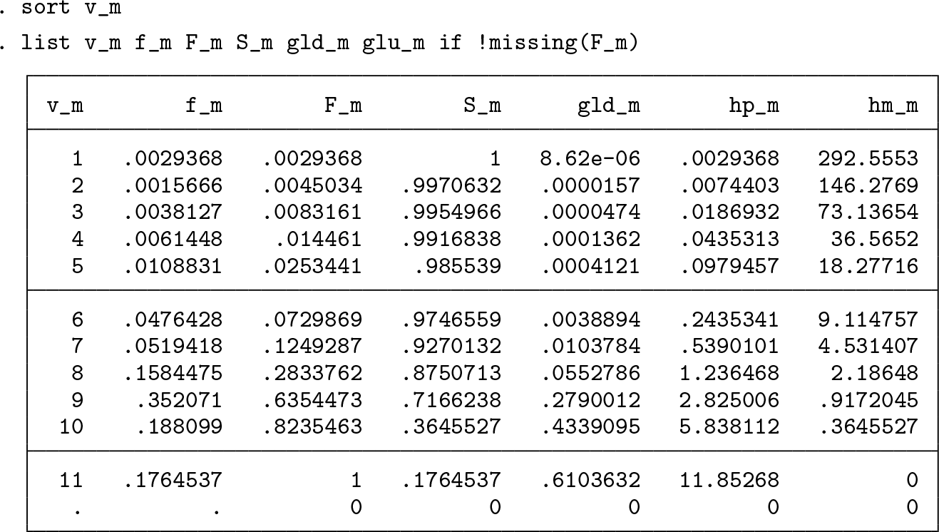
Figure 1 shows the CDFs for the three marital status groups. The code used to produce the graph follows below. (Stata 14 users should omit the “%55”, which refers to a transparency option introduced in Stata 15.)

Figure 1.

Cumulative distribution functions (CDFs) for life satisfaction, by marital status group

We can see immediately that 9 is the median value of ls for all three groups (the value where cumulative population share, p = 0.5). The CDF for married adults lies everywhere on or below the CDFs for the other two groups (F-dominance), so we can say that married adults have higher average life satisfaction than the other two groups, regardless of the scale used. The CDFs for the SNM and SDW groups cross, so there is no F-dominance result. However, there is S-dominance. Below the median, the

CDF for the SDW group is further from the median than the CDF for the SNM group, and the reverse is the case above the median. Thus, there is greater polarization in the distribution of life satisfaction among the SDW group than among the SNM group according to all standard polarization indices—including all members of the ANY(a, b) and P2(e) families of indices.

To check for unanimous rankings by Cowell–Flachaire and J indices, I focus on the peer-inclusive downward-looking definition of status for brevity. Figure 2 shows the results of the three pairwise comparisons between groups. Below, I show the code used for the married and SDW groups’ comparison. Analogous code for the other two pairwise comparisons followed by graph combine produced figure 2.

Figure 2.

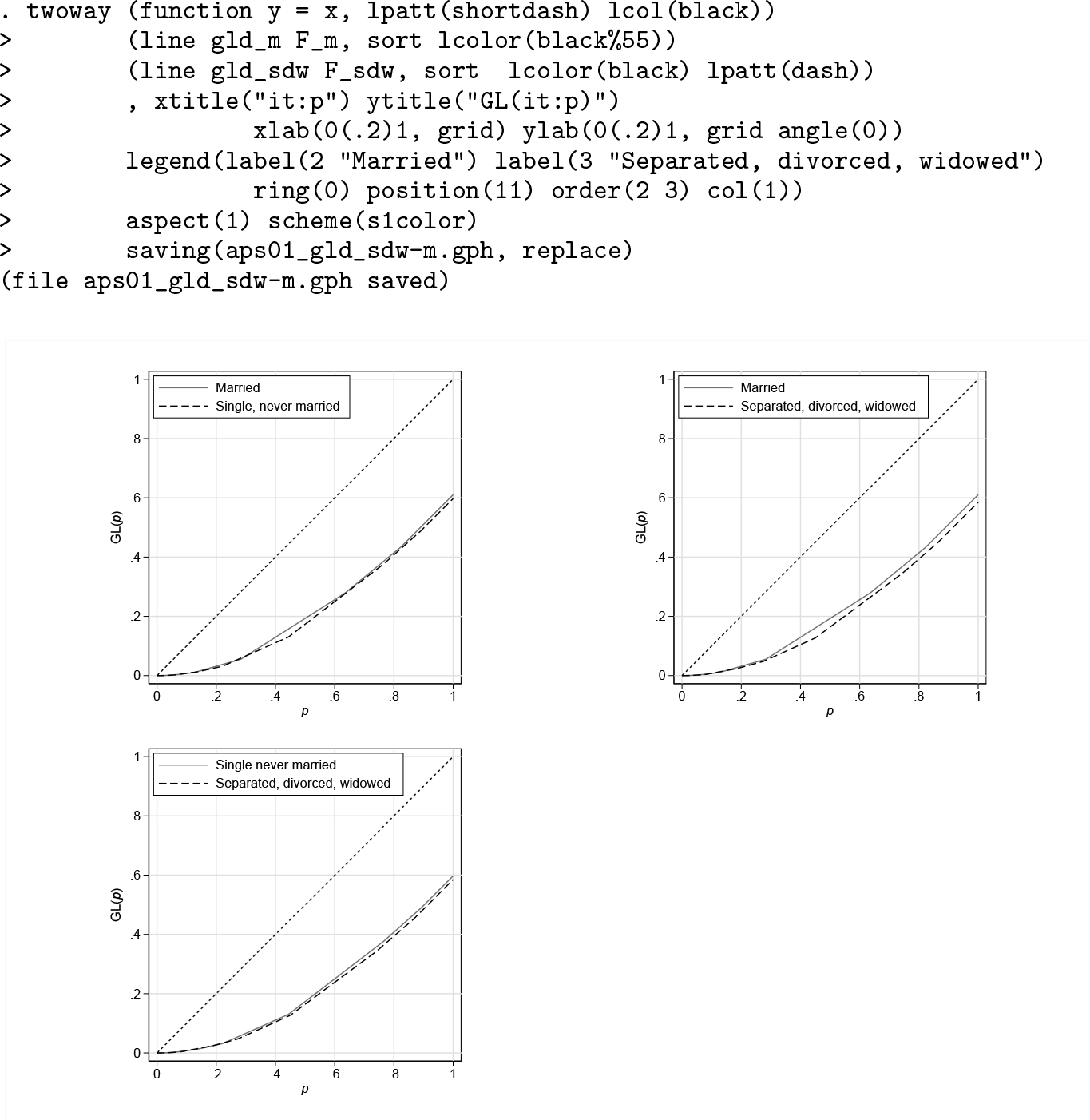
Generalized Lorenz curve comparisons for life satisfaction, by marital status group

All three pairwise comparisons reveal dominance. The clearest result, in the sense that the gap between the GL curves for status is greatest, is in the top-right picture: life satisfaction is more unequal for the SDW group than the married group according to all Cowell–Flachaire indices and the J index. The other two charts show that inequality is greater among the SNM group than the married group and among the SDW group compared with the SNM group. Thus, there is an unambiguous ranking from highest to lowest inequality according to all Cowell–Flachaire indices and J, with the SNM group the most unequal, the married group the least unequal, and the SDW group in between.

Figure 3 summarizes checks of Gravel, Magdalou, and Moyes’s (Forthcoming) dual dominance criteria based on H ⁺ and H⁻ curve comparisons. The code used for the comparison of H ⁺ curves for married and single, never-married groups is shown below. Analogous code for the other two pairwise H ⁺ comparisons and for the three H⁻ comparisons followed by graph combine produced figure 3.

Figure 3.

H ⁺ and H⁻ curve comparisons for life satisfaction, by marital status group

Recall that for Gravel, Magdalou, and Moyes’s dual dominance criteria to be satisfied, we need to find the H ⁺ and H⁻ curves for one group nowhere above the corresponding curves for another group. For these data, the orderings of the groups according to the H ⁺ criterion are the same as the orderings by the F-dominance criterion (because F-dominance implies H ⁺ dominance). See the charts on the left-hand side of figure 3. However, there is dual dominance in only one case. The distribution of life satisfaction among the single, never-married group is more equal than the distribution among the separated, divorced, widowed group: the H ⁺ and H⁻ curves for the former group are nowhere below those for the latter group. This ordering of the two groups, based on Hammond transfer principles, is the same as their ordering according to the S-dominance criterion (referring to greater polarization about the median) and is also the same as their GL dominance ordering (see figure 2).

4.3 Indices of polarization and inequality

Estimates of specific polarization and inequality indices are consistent with this dominance result and also the S-dominance result cited earlier (the SDW group is more polarized about the median than the SNM group). Specific indices are also useful for deriving inequality and polarization orderings when there is no dominance result and, of course, can be used to place a number on the magnitude of differences. To illustrate these points, I present estimates of a selection of inequality indices [I(α) for α = 0, 0.25, 0.5, 0.75, 0.9; and J; all using a peer-inclusive downward-looking status definition] and three polarization indices, ANY(1, 1), the top-sensitive ANY(4, 1), and the bottom-sensitive ANY(1, 4). In addition, I show how one can derive standard errors for the indices using Saigo, Shao, and Sitter’s (2001) repeated half-sample bootstrap using Van Kerm’s (2013) rhsbsample (available from the SSC archive), with 500 bootstrap replications in this case. With the APS’s very large sample size, the indices are going to be precisely estimated and confidence intervals narrow, even for subgroup calculations, but this is not generally the case with survey data. (See Jenkins [Forthcoming] for examples.) Hence, this code may be usefully applied in other contexts.

The code below shows the derivations for the married group. First, I drop observations with missing values. Second, I use rhsbsample to create the bootstrap sample weights. Third, I svyset the data. If survey design variables other than weights—primary sampling unit and strata variables—had been available, this is where they would have been cited. Fourth, I call ineqord using the svy bootstrap prefix command. Observe that I use the alpha(0.9) option to derive estimates of the Cowell–Flachaire indices, I(α), for values of α spanning its range. (I also derived estimates for more polarization indices than I cited earlier, just in case I needed them.) The “d” suffix on the estimates’ names reminds us that I am using Cowell and Flachaire’s peer-inclusive downward-looking status definition. Finally, I save the estimates of indices, standard errors, and confidence intervals to a dataset using Newson’s (2003) parmest utility command (latest version available from the SSC archive).

I repeated this code for the SNM and SDW groups as well, specifying different arguments for parmest‘s idn(.) option in each case to separately identify the estimates for the three marital status groups when I combined the three datasets using append. Using the combined-estimates dataset, we can straightforwardly summarize differences across groups, by index, in graphical form. See figure 4 created by first creating graphs for each index and then using graph combine. Here is the code used to display the estimates for I(0):

All indices are very precisely estimated, and all between-group differences are statistically significantly different from 0.

The rankings of marital status subgroups in figure 3 are of course consistent with the dominance results discussed earlier. However, there was no S-dominance result for the polarization comparisons between the married group and each of the other two groups, so index values are valuable for providing a polarization ranking. Interestingly, figure 4 shows that this depends on the index chosen. For ANY(1, 1) and ANY(1, 4), the ranking is the same as for the inequality indices. However, for top-sensitive index, ANY(4, 1), the married group shows the greatest polarization rather than the lowest. What is driving this result is that the married group has relatively large fractions of responses in the top-two life-satisfaction scale categories in contrast with the other two groups (see the tabulation of life satisfaction by marital status shown earlier).

Indices also tell us about the magnitudes of differences across groups. As it happens, the I(α) and J indices provide similar estimates. For example, all of them indicate that the difference in life satisfaction inequality between the most unequal group (SDW) and the least unequal group (married) is around 7%. More marked differences are apparent for the ANY polarization indices. For example, for ANY(1, 1), which is also the average jump index, the difference in polarization between the SDW and married groups is around 39%, whereas for ANY(1, 4), it is around 17%. For ANY(4, 1), it is −20%.

Figure 4.

Indices of life-satisfaction inequality and polarization, by marital status group

4.4 Using grouped data with ineqord

ineqord is designed for use with datasets containing individual-level responses, but it is straightforward to also use it if only grouped response data are available, specifically, if one has information on the number of individuals reporting each response level (or fraction of individuals) or the empirical CDF.

For example, Abul Naga and Yalcin (2008, table 2) report the empirical CDF for self-reported health status recorded on a 5-level scale (“very bad”, “bad”, “so so”, “good”, “very good”) for each of seven statistical areas in Switzerland. The empirical CDF for the Central region can be reproduced using the following code to characterize the distribution of responses:

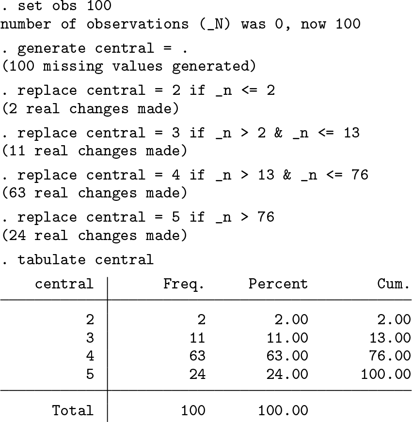
No individuals in the Central region reported “very bad” health status and so simply typing ineqord central will produce incorrect results, for the reasons discussed earlier. However, typing ineqord central, nlevels(5) produces estimates that are the same as those reported by Abul Naga and Yalcin (2008, table 4). Application of analogous code using information about the empirical CDFs for the other six regions reproduces the estimates for the regions reported in Abul Naga and Yalcin’s table 4, as well as provides estimates for other indices that they did not consider. With appropriate use of ineqord options, it is easy to also derive the outputs required to undertake dominance checks.

Using the same grouped-data approach, I have verified that ineqord produces the same estimates of ANY polarization indices as reported by Madden (2010) for selfreported health status in Ireland in each year 2003–2006. I can also reproduce the estimates of the Blair–Lacy 1 − l ² polarization index shown by Blair and Lacy (2000, table 2) once I account for some typographical errors (estimates of l ² are reported in the wrong table rows).

5 Summary and conclusions

The personal well-being of individuals is increasingly being measured using questions requiring responses on a Likert-type scale. Life satisfaction and self-assessed health status are leading examples of these measures, and they yield distributions of ordinal data. To compare such distributions across groups of individuals or over time, we should not apply the toolbox of methods developed for cardinal variables such as income. These methods rely on the mean as a reference point, but changing the scale in the ordinal data case can change the orderings of distributions according to their means or other measures based on the mean, including conventional inequality indices. Thus, we should use an analogous toolbox that accounts for the ordinal nature of the responses. This article reviewed these methods and introduced a new command, ineqord, for undertaking distributional comparisons. As the empirical illustrations demonstrated, ineqord can be used for dominance checks as well as for estimation of indices of polarization and inequality.