
Abstract
Cluster randomized trials, where clusters (for example, schools or clinics) are randomized to comparison arms but measurements are taken on individuals, are commonly used to evaluate interventions in public health, education, and the social sciences. Analysis is often conducted on individual-level outcomes, and such analysis methods must consider that outcomes for members of the same cluster tend to be more similar than outcomes for members of other clusters. A popular individual-level analysis technique is generalized estimating equations (GEE). However, it is common to randomize a small number of clusters (for example, 30 or fewer), and in this case, the GEE standard errors obtained from the sandwich variance estimator will be biased, leading to inflated type I errors. Some bias-corrected standard errors have been proposed and studied to account for this finite-sample bias, but none has yet been implemented in Stata. In this article, we describe several popular bias corrections to the robust sandwich variance. We then introduce our newly created command,
Keywords
1 Introduction
The cluster randomized trial (CRT) is a study design used in many fields of research. In a CRT, randomization to intervention arms is carried out at the cluster level (for example, schools or clinics) and outcomes are assessed for each member of each cluster. The cluster randomization design is typically chosen when there is a high chance of treatment spillover across study arms, when the intervention is group based, or when individual randomization is not feasible (Turner et al. 2017a). For example, a recent trial in Ghana is evaluating an intervention designed to assist mothers with children that are under two years old to become more resilient and more effectively manage daily stress (Baumgartner 2018). The trial adopts a cluster randomized design because the intervention is designed to be delivered to groups of women. As another example, in the Thinking Healthy Program Peer-Delivered Plus study, the researchers recruited depressed women in their third trimester of pregnancy from 40 villages in Pakistan, with each village then being randomized to receive either the intervention or enhanced usual care (Sikander et al. 2015; Turner et al. 2016). Because this was a public health intervention delivered by community health workers, the risk of contamination (that is, the intervention being transmitted to women in the control group) would be too high if individual women were randomized, given that many of the women within each village live relatively close to one another.
Randomizing clusters instead of individuals poses unique challenges to the data analyses because the outcomes for members of the same cluster tend to be more similar than those for members of different clusters. The intraclass correlation coefficient (ICC) is a quantity that measures the degree of similarity for within-cluster observations and plays a central role in the design and analysis of CRTs (Murray 1998). Appropriate statistical methods used for trial analyses should properly reflect the within-cluster correlation and mainly include two classes of regression models: the cluster-specific (conditional) model and the population-averaged (marginal) model (Fitzmaurice, Laird, and Ware 2011). Although each modeling strategy has its own advantages, an important distinction between them is the difference in interpretation of the regression parameters (Preisser et al. 2003). A conditional model, such as the generalized linear mixed model, induces the within-cluster correlation through the latent random effects. Thus, the interpretation of the treatment effect is the average change in outcomes from control to intervention, conditional on the unobserved random effect. By contrast, marginal models separately specify a mean structure and a “working” correlation structure, and the interpretation of the corresponding treatment effect is the average change in outcomes due to intervention among the population defined by all participating clusters. Because CRTs are often conducted to evaluate public health intervention and inform policy decision, the marginal model carries a straightforward population-averaged interpretation and may be preferred (Li, Turner, and Preisser 2018). Furthermore, the estimation and inference of marginal models are often conducted through generalized estimating equations (GEE) (Liang and Zeger 1986), a multivariate extension of the quasilikelihood inference (Wedderburn 1974).
In addition to straightforward interpretation of estimated model parameters, GEE maintains a robustness property in that the treatment-effects estimates are consistent even if the working correlation model deviates from the true correlation model. In this case, the sandwich variance estimator (Liang and Zeger 1986) remains consistent to the true variance. However, the approximate unbiasedness of the sandwich variance holds only when there are many clusters (a rule of thumb is ≥ 30, although this rule is sometimes given as ≥ 40 or even ≥ 50), whereas a frequent practical limitation of CRTs is that few clusters are available, because of resource constraints. In fact, a recent review by Fiero et al. (2016) found that, of the 86 studies included, about 50% randomized 24 or fewer clusters. In CRTs related to cancer published between 2002 and 2006, Murray et al. (2008) found similar results, with about 50% randomizing 24 or fewer clusters. Additionally, in their review of 300 CRTs published between 2000 and 2008, Ivers et al. (2011) found that, of the 285 studies reporting the number of clusters randomized, at least 50% randomized 21 or fewer clusters. Often, randomizing such few clusters is done because every cluster included in the study adds strain to limited financial and human resources. For example, in a study examining an intervention targeted at early childhood development among HIV-exposed children in Cameroon, only 10 total clusters were randomized because of resource and practical limitations (Baumgartner 2017).
When fewer than 30 to 40 clusters are randomized, the GEE sandwich variance estimator tends to be biased toward zero, leading to inflated type I error rates when testing for the intervention effect (Hayes and Moulton 2009). Proper analyses of CRTs should account for such finite-sample bias in variance estimation and adopt the bias-corrected variance estimator (Turner et al. 2017b). Several proposals for correcting such finite-sample bias have appeared in the statistical literature; see, for example, Mancl and DeRouen (2001); Kauermann and Carroll (2001); Fay and Graubard (2001) among others. These proposals have existed for over 15 years, but to our knowledge none has yet been implemented in Stata. Introducing the bias-corrected variance estimators to Stata has significant practical implications because Stata is a popular software tool for CRT analysts. The availability of this routine will help promote better statistical practice by allowing future analysts to report appropriate p-values and confidence intervals.
The remainder of this article is organized into four sections. In section 2, we introduce the theory of bias-corrected sandwich variance estimators for GEE analyses of CRTs. In section 3, we present our newly created command,
2 Statistical methods
2.1 GEE
We consider a parallel-arm CRT consisting of n clusters allocated into two intervention arms and note that the methods are generalizable to CRTs with more than two intervention arms. The outcome of each participant is typically measured at the end of the study and represented by Yij
(i = 1,…, n, j = 1,…, mi
), where mi
is the number of individuals in cluster i. We denote the p × 1 design vector by
Let
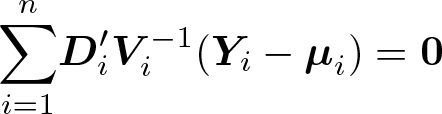
The GEE estimators
with a Newton-type algorithm implemented in the
where
2.2 Bias-corrected sandwich variance estimators
A practical limitation of CRTs is that fewer than 30 to 40 clusters are often randomized, mainly because of availability or resource constraints (Ivers et al. 2011; Fiero et al. 2016). When the number of clusters is small, it is known that the residuals,
Define the cluster leverage to be

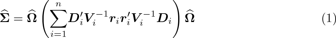
Because elements of

Mancl and DeRouen (2001) devised a similar bias correction by using

Because elements of the cluster leverage
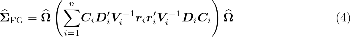
where

where
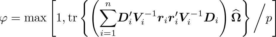
quantifies the design effect (Morel 1989). Of note, the additive bias correction (5) ensures a positive-definite covariance matrix, while the multiplicative bias corrections (2), (3), and (4) do not guarantee the positive definiteness of the estimated covariance (Morel, Bokossa, and Neerchal 2003), which was argued to be an additional benefit of (5). Once the variance estimator for the intervention effect is obtained using one of these bias-corrected variance formulas, we could conduct a test of no intervention effect by using the standard Wald z test or the Wald t test with DF n − p.
2.3 Computations with large cluster sizes
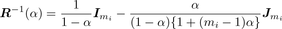
When the cluster sizes mi become large (greater than 1,000), calculation of the biascorrected variance estimators may become computationally inefficient because of numerical inversion of large matrices. To alleviate such a concern, we first note that a closed-form expression is available for the inverse of the exchangeable correlation structure (Li, Turner, and Preisser 2018; Li et al. 2019) and is given by
Furthermore, Preisser, Qaqish, and Perin (2008) noted that inverting the asymmetric matrix
3 The xtgeebcv command
The
The user should first specify a variable list (varlist) with an outcome (dependent) variable followed by predictor (independent) variables, just as one would do with the
Inside the command, the user-supplied data are passed to the
The design matrix, coefficient estimates, and variance–covariance matrix of the parameters output by the
3.1 Syntax
varlist contains the regression specification: the dependent variable (outcome) followed by independent variables (predictors). Note that all categorical variables with more than two levels will need to be dummy coded by the user before supplying them to the command.
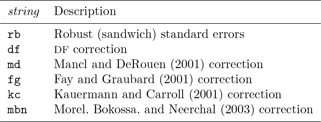
3.2 Options
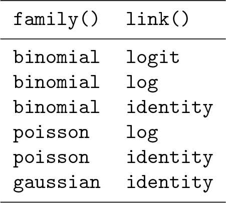
xtgee_options are any of the options documented in [XT]
4 Illustrative examples
In this section, we illustrate the use of
4.1 Equal-sized clusters
First, we simulated correlated binary data using the method of Lunn and Davies (1998). We created a dataset with 80 clusters, 2 treatment arms (treatment and control), and exactly 14 individuals per cluster. The data were simulated so that the probability of outcome in the treatment group would be approximately 65%, while the probability in the control group would be 45%. This corresponds to a risk ratio of 1.44 or an odds ratio of 2.08, comparing treatment with control. After this, 20 clusters were randomly sampled from the dataset, 10 in treatment and 10 in control, to mimic a CRT with few clusters. To obtain an estimate of the risk ratio with Mancl–DeRouen finite-sample correction to the standard error, we use a log-binomial regression model by specifying a binomial distribution with a log-link function.
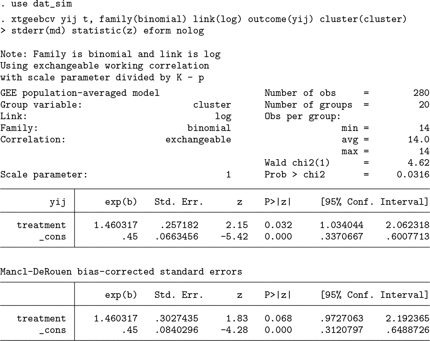
The first set of estimates comes from the GEE model with the scale parameter estimated using the n − p DF, as discussed in section 3, and uses the conventional (model-based) standard errors. The second table gives the parameter estimates and Mancl–DeRouen corrected standard errors. We chose this bias correction because Lu et al. (2007) suggested that it performs adequately along with a z test if the number of clusters is in the range of 10 to 20.
The variance–covariance matrix of the parameter estimates for the chosen finitesample correction is stored in
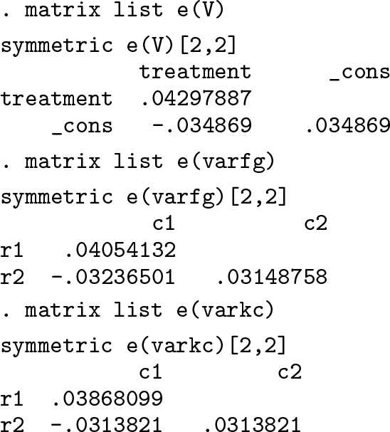
Below, we also output the robust standard errors not multiplied by K/(K − 1), where K is the number of clusters.
2
Because the bias corrections are applied to this robust (sandwich) variance, we want to compare the standard-error estimates of the Mancl–DeRouen finite-sample correction with this robust variance, rather than with the conventional (model-based) standard-error estimates output from
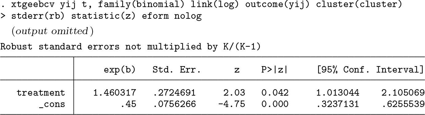
In this instance, if the researchers were using a strict 0.05 cutoff for significance, their conclusion about the statistical significance of the treatment effect would change if using the bias-corrected standard errors compared with the robust standard-error estimates.
4.2 Unequal-sized clusters
In this section, we use data from the MEME kwa Vijana (MKV) CRT in Tanzania, which is described in Hayes and Moulton (2009, 23) and is also published in Ross et al. (2007). The data are publicly available online (Hayes and Moulton 2016). In brief, the goal of the trial was to evaluate the impact of a sexual health intervention on various HIV-related outcomes. The publicly available dataset includes data from male participants at follow-up, with the main outcome provided being “good knowledge of HIV acquisition”, a binary variable. In this dataset, there are 20 communities that were randomized to receive either intervention or “standard activities”. The number of participants per community ranges from 169 to 257, with a mean of 205 and a standard deviation of 26.3. The coefficient of variation of cluster sizes is 0.128. In this dataset, 65.3% of the intervention group has good knowledge of HIV acquisition at follow-up versus 44.9% in control, corresponding to an (unadjusted) odds ratio of 2.32 and risk ratio of 1.46.
The goal of the analysis is to estimate the odds ratio comparing intervention with control, while demonstrating the use of the Kauermann–Carroll finite-sample correction. In addition to including intervention group (
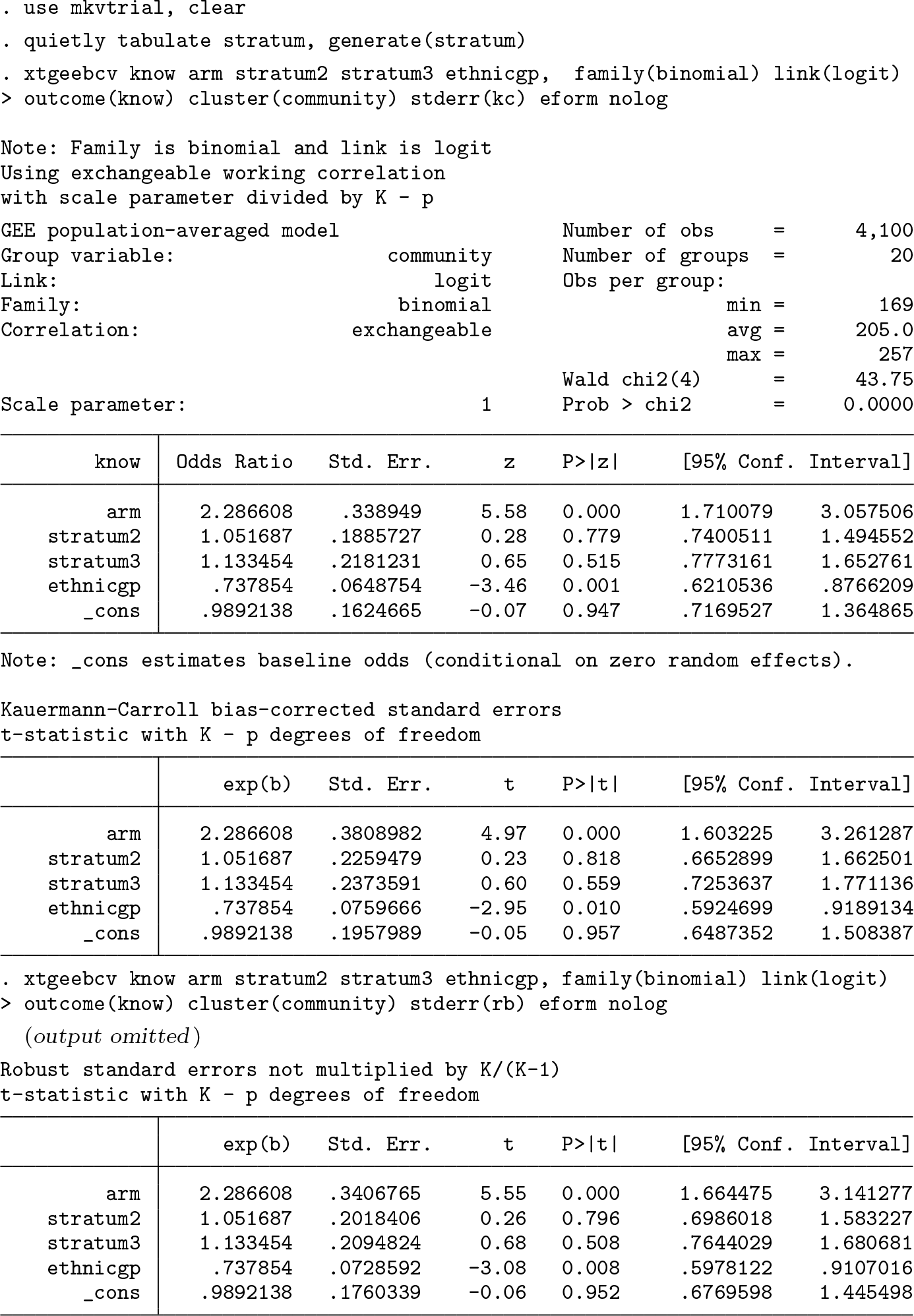
In this case, with 20 clusters and many participants per cluster, although the finitesample correction inflates the standard error by about 12% above the robust standard errors, any conclusion about significance of the effect based on the p-value would not change.
To see the potential impact of finite-sample corrections, suppose the researchers are interested in the intervention effect only in stratum 2. To this end, we subset the dataset to the 8 communities in stratum 2. This dataset has cluster sizes ranging from 187 to 243, with a mean of 214 and standard deviation of 21.1, which gives a coefficient of variation of cluster sizes of 0.099. In this dataset, 63.2% of the intervention group has good knowledge of HIV acquisition at follow-up versus 45.7% in control. Because we have subset on the stratum, we no longer adjust for this variable.
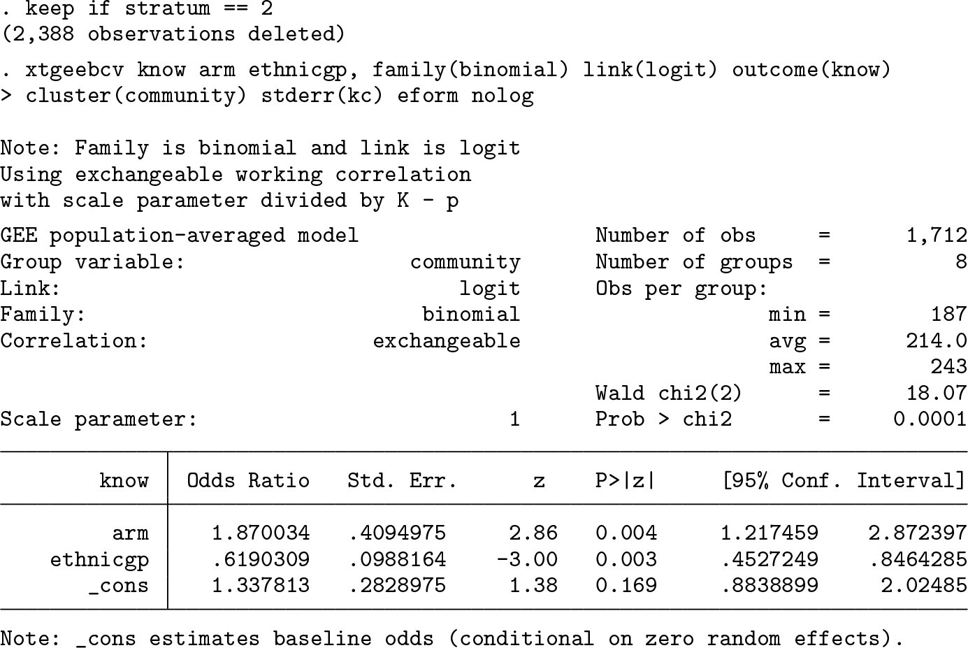
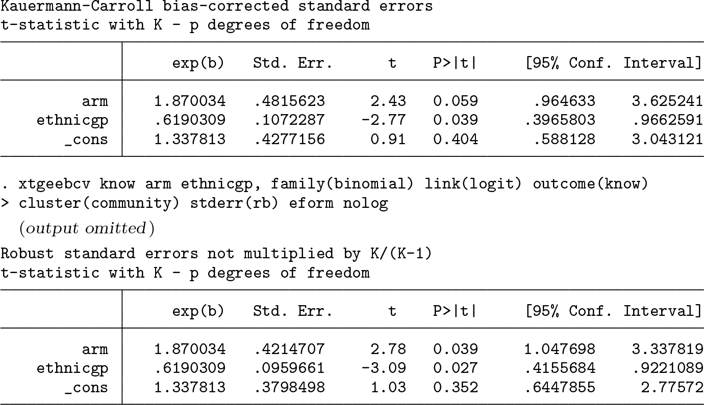
From the GEE model with robust standard errors, we estimate an adjusted odds ratio of 1.87 (95% confidence interval [1.05, 3.34]). This estimate is significant at the 0.05 level. After we apply the Kauermann–Carroll bias correction to the robust standard errors, inflating the standard error of the intervention effect by 14.3%, the 95% confidence interval widens to [0.96, 3.63]. The Kauermann–Carroll correction and the t-test statistic were chosen in this case given that Li and Redden (2015) suggested that they maintain close to the nominal type I error rate when the coefficient of variation of cluster sizes is less than 0.6. Compared with the p-value associated with the robust standard errors (p = 0.039), this estimate is not significant at the 0.05 level (p = 0.059).
5 Discussion
Many CRTs randomize fewer than 40 clusters, and cluster size is often highly variable. Many researchers use Stata to analyze their CRTs. Current GEE routines in Stata may not properly account for the small-sample bias in the robust standard errors and so may risk an inflated type I error rate when used in the analysis of small CRTs. We have introduced the
Although we have enabled the implementation of bias-corrected sandwich variance estimators in Stata, we have not attempted to make specific recommendations as to which correction works best in small CRTs. Several suggestions have been put forward in the statistical literature. For example, Li et al. (2017) found that the Wald t test with
There are some limitations to
7 Programs and supplemental materials
Supplemental Material, st0599 - xtgeebcv: A command for bias-corrected sandwich variance estimation for GEE analyses of cluster randomized trials
Supplemental Material, st0599 for xtgeebcv: A command for bias-corrected sandwich variance estimation for GEE analyses of cluster randomized trials by John A. Gallis, Fan Li and Elizabeth L. Turner in The Stata Journal
Footnotes
6 Acknowledgments
The authors would like to thank Alyssa Platt, Joe Egger, and Ryan Simmons of the Duke Global Health Institute Research Design and Analysis Core for testing and providing feedback on the programs. We would also like to thank an anonymous reviewer whose comments on a previous version of this manuscript helped improve the final version. This research was funded in part by National Institutes of Health grant R01 HD075875 (principal investigator [PI]: Dr. Joanna Maselko). In addition, the development of the command
7 Programs and supplemental materials
To install a snapshot of the corresponding software files as they existed at the time of publication of this article, type
Notes
References
Supplementary Material
Please find the following supplemental material available below.
For Open Access articles published under a Creative Commons License, all supplemental material carries the same license as the article it is associated with.
For non-Open Access articles published, all supplemental material carries a non-exclusive license, and permission requests for re-use of supplemental material or any part of supplemental material shall be sent directly to the copyright owner as specified in the copyright notice associated with the article.