feologit: A new command for fitting fixed-effects ordered logit models

Abstract

In this article, we describe how to fit panel-data ordered logit models with fixed effects using the new community-contributed command feologit. Fixed-effects models are increasingly popular for estimating causal effects in the social sciences because they flexibly control for unobserved time-invariant heterogeneity. The ordered logit model is the standard model for ordered dependent variables, and this command is the first in Stata specifically for this model with fixed effects. The command includes a choice between two estimators, the blowup and cluster (BUC) estimator introduced in Baetschmann, Staub, and Winkelmann (2015, Journal of the Royal Statistical Society, Series A 178: 685–703) and the BUC-τ estimator in Baetschmann (2012, Economics Letters 115: 416–418). Baetschmann, Staub, and Winkelmann (2015) showed that the BUC estimator has good properties and is almost as efficient as more complex estimators such as generalized method-of-moments and empirical likelihood estimators. The command and model interpretations are illustrated with an analysis of the effect of parenthood on life satisfaction using data from the German Socio-Economic Panel.

1 Introduction

While originating in the biometrics literature, regression models for ordered responses are now ubiquitous in the social sciences (Boes and Winkelmann 2006). One factor contributing to the widespread use of ordered responses is that Likert-type scales are the default way in which individual, household, and firm surveys collect information on issues that are otherwise difficult to measure, such as attitudes and beliefs. By far, the most common cross-sectional regression models for ordered responses are the ordered logit and ordered probit models. When analyzing ordinal panel data, researchers are frequently interested in applying extensions of these models that somehow account for the longitudinal nature of the data. The simplest approach, which we consider in this article, is specifying an additional unobservable individual-specific error term. Under the assumptions that this error term is normally distributed and independent of the regressors, the models are known as the random-effects ordered logit or random-effects ordered probit (see, for example, Cameron and Trivedi [2005]), and they are implemented in Stata with the commands xtologit and xtoprobit, respectively.

Often, however, these distributional and independence assumptions on the individual-specific error term are undesirable. Fixed-effects models relax them: the distribution of the individual-specific error term and its dependence on the regressors are left completely unrestricted (compare, for example, Wooldridge [2010]). This feature of fixed-effects models is useful for the estimation of causal effects because it accounts for any potential endogeneity stemming from time-invariant characteristics. But because no default approach for fitting fixed-effects models for ordered responses exists, researchers are often faced with the choice of either fitting linear models, which are often inappropriate for ordinal data, or fitting random-effects ordered logit or probit models, which impose the strong assumptions mentioned above.

Because a fixed-effects estimator exists for the binary logit model, several different estimators for fixed-effects ordered logit models can be obtained using the binary logit model as a building block: the ordinal response variable can be transformed into binary responses, which then can be used for estimation and combined back differently to provide a single set of estimates. For the ordered probit model, in contrast, a similar approach is infeasible because no fixed-effects estimator for the binary probit model exists. Baetschmann, Staub, and Winkelmann (2015) studied several approaches available for the fixed-effects ordered logit model and showed that the so-called blow-up and cluster (BUC) estimator has good properties and is almost as efficient as more complex estimators such as generalized method-of-moments and empirical likelihood estimators. In this article, we discuss the BUC estimator as well as a more restricted version of it that makes it possible to fit additional model parameters—the BUC-τ estimator introduced in Baetschmann (2012)—and show how these estimators can be implemented in Stata using the community-contributed command feologit.

An integral part of our discussion focuses on the various potential objects of interest in this model, such as marginal effects (MEs), odds ratios, etc., and on whether they can or cannot be estimated, and if so, how. We further introduce a new specification test of the more restrictive assumptions relating to the additional threshold parameters estimated by BUC-τ. The test is simple to implement, and we show in an example using Stata syntax how BUC and BUC-τ estimates can be used to this end. Finally, we illustrate the use of feologit and the interpretation of the estimates in an application of the effect of motherhood on women’s life satisfaction, which uses data from the German Socio-Economic Panel (SOEP).

We review the fixed-effects ordered logit model and the BUC and BUC-τ estimators in the next section. The syntax for feologit is presented in section 3.1. Next, section 4 gives a guide on how to interpret estimates. Section 5 exemplifies the use of feologit and possible interpretations of the estimates in the application to life satisfaction and provides a test of the BUC versus BUC-τ estimates. Section 5 offers some concluding remarks.

2 Fixed-effects ordered logit models

The fixed-effects ordered logit model uses the latent variable y ^∗ to relate the observable characteristics x to the observable ordered dependent variable y, which can take values 1,…, K. The latent variable $y_{it}^{\ast }$ for individual i at time t depends linearly on x _it and the two unobservable characteristics α_i and ε_it :

$y_{it}^{\ast }={x^{\prime }}_{it}\beta +{\alpha }_i+{\epsilon }_{it}i=1,\dots ,N\hspace{0.17em}\hspace{0.17em}t=1,\dots ,T$

The vector of covariates x _it does not include an intercept because the α_i act as individual-specific intercepts. We use a balanced panel for notational simplicity; but extending the model to imbalanced panels (t = 1,…, T_i ) is trivial, and the application in section 5 uses such an imbalanced panel. The time-invariant, individual-specific part of the unobservables (α_i ) is called the fixed effect and can statistically depend on x _it . The following observation rule ties the latent variable $y_{it}^{\ast }$ to the observed ordered variable y_it through the thresholds τ_ik :

$y_{it}=k\hspace{0.17em}\hspace{0.17em}\text{if}\hspace{0.17em}\hspace{0.17em}{\tau }_{ik}<y_{it}^{\ast }\le {\tau }_{ik+1}\hspace{0.17em}\hspace{0.17em}\hspace{0.17em}k=1,\dots ,K$

In the most flexible version of the model, the thresholds can vary between individuals, as indicated by the subscript i in τ_ik . Besides the stipulation of the lowest and highest thresholds as plus and minus infinity, the only assumption about the individual-specific thresholds is that they are increasing for each person:

${\tau }_i{ }_1=-\infty ;\hspace{0.17em}\hspace{0.17em}\hspace{0.17em}-\infty <{\tau }_{ik}<{\tau }_{ik}{ }_{+1}<\infty ,\hspace{0.17em}\hspace{0.17em}\forall k=2,\dots ,K-1;\hspace{0.17em}\hspace{0.17em}\hspace{0.17em}\hspace{0.17em}{\tau }_{iK}{ }_{+1}=\infty$

1

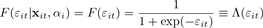
Moreover, the fixed-effects ordered logit model assumes that the time-varying unobservable terms, ε_it , are independent and identically distributed with standard logistic cumulative density function, hence the name of the model:

$F\left({\epsilon }_{it}|x_{it},{\alpha }_i\right)=F({\epsilon }_{it})=\frac{1}{1+\exp \left(-{\epsilon }_{it}\right)}\equiv \Lambda \left({\epsilon }_{it}\right)$

The probability of observing outcome k for individual i at time t is therefore

$\text{Pr}\left(y_{it}=k|x_{it},{\alpha }_i\right)=\Lambda \left({\tau }_{ik}{ }_{+1}-{x^{\prime }}_{it}\beta -{\alpha }_i\right)-\Lambda \left({\tau }_{ik}-{x^{\prime }}_{it}\beta -{\alpha }_i\right)$

2

This probability depends on x _it and β , the parameter of primary interest. However, it also depends on α_i , τ_ik , and τ_{ik +1}. As can be seen from (2), without further assumptions on the thresholds, only τ_ik − α_i ≡ α_ik is identified because we can always define ${\tilde{\tau }}_{ik}={\tau }_{ik}+\eta$ and ${\tilde{\alpha }}_i={\alpha }_i-\eta$ for any η ∊ $ℝ$ . ¹

Direct estimation of α_ik is difficult. Generally, estimation of α_ik uses only information of the T observations of individual i. Thus, if the time dimension T is fixed—as is generally assumed in short panels—there are only a finite number of observations to estimate α_ik even when the total number of observations NT grows to infinity. Consequently, the fixed effects α_ik cannot be estimated consistently, and, in general, their inconsistency spills over to inconsistency of β , the parameters common to all observations. This situation is known as the incidental parameters problem (Neyman and Scott 1948; Lancaster 2000). In short panels, the resulting bias in $\widehat{\beta }$ can be substantial (Abrevaya 1997; Greene 2004). A consistent estimator of β can be obtained by collapsing y_it into a binary variable and then applying the well-known conditional maximum likelihood (CML) estimator (Andersen 1970; Chamberlain 1980).

2.1 CML estimator

The CML estimator is well known. But because the BUC estimator for the fixed-effects ordered logit model is based on the CML, we present it in some detail to fix notation. In Stata, this estimator is implemented in the command clogit and in the panel-data command xtlogit with the option fe, which relies on clogit. Similarly, feologit also relies on clogit.

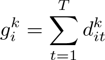
Let $d_{it}^k$ denote the binary variable that results from dichotomizing the ordered variable at the cutoff point k: $d_{it}^k=1\left(y_{it}\ge k\right)$ . This is the dependent variable of the CML estimator. Let

$g_i^k={\displaystyle \sum _{t=1}^T{d}_{it}^k}$

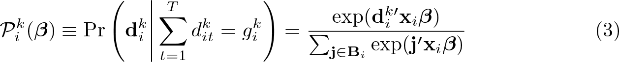
be the observed number of ones of the dependent variable for individual i. Now, consider the probability of observing $d_i^k={\left(d_{i1}^k,\dots ,d_{iT}^k\right)}^{\prime }$ conditional on observing $g_i^k$ ones. It can be shown that this probability is

$P_i^k\left(\beta \right)\equiv \mathrm{Pr}\left(d_i^k|{\displaystyle \sum _{t=1}^T{d}_i^k=g_i^k}\right)=\frac{\exp \left(d_i^{k\prime }{x}_i\beta \right)}{{\sum }_{j\in B_i}\exp \left(j\prime x_i\beta \right)}$

3

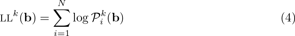
where j denotes a vector of dimension T with each element j_t equal to 0 or 1 and with ${\displaystyle {\sum }_{t=1}^T{j}_t}=g_i^k$ . Further, B _i denotes the set of all possible j-vectors with $g_i^k$ ones and $T-g_i^k$ zeros. There are $\left(\begin{array}{c}T\\ g_i^k\end{array}\right) =T!/\left\{g_i^k!(T-g_i^k)!\right\}$ such combinations. Crucially, this probability (3) does not depend on α_i and the thresholds. Chamberlain (1980) showed that maximizing the conditional log likelihood (LL)

${\text{LL}}^k\left(b\right)={\displaystyle \sum _{i=1}^N\log P_i^k}\left(b\right)$

4

results in a consistent estimator for β . Therefore, β of the fixed-effects ordered logit model can be fit by first dichotomizing the ordered dependent variable into a binary one and then applying the standard CML estimator. However, different cutoff points k can be used, and using only one of them leads to loss of information and, therefore, to inefficiency. Further details of the CML estimator such as first-order conditions and asymptotic variance can be found, for example, in Baetschmann, Staub, and Winkelmann (2015).

2.2 BUC estimator

Several ideas exist to combine the information of the CML estimators obtained from dichotomizing samples at different cutoff points (see Baetschmann, Staub, and Winkelmann [2015]). The BUC estimator presented here combines the LL functions resulting from different cutoff points, leading to a one-step estimator of β . The LL function for this estimator is

${\text{LL}}^{\text{BUC}}(b)={\displaystyle \sum _{k=2}^K{\text{LL}}^k(b)}$

5

where LL ^k (b) is defined as in (4) and the BUC estimator is the one that maximizes (5). It can also be regarded as a restricted CML estimator because it imposes the restriction that ${\widehat{\beta }}^2=\cdots ={\widehat{\beta }}^K$ . We call this the BUC estimator because this describes how the estimator is implemented: first, every individual’s observations in the sample are replaced with K−1 copies or clones of itself (“blow up” the sample size); and, then, each clone is dichotomized at a different cutoff point. We then use the entire inflated sample to estimate β by applying the CML estimator. Because the clones of the same individual are not independent of each other, we have to compute standard errors that are clustered at the individual level. Baetschmann, Staub, and Winkelmann (2015) have shown that combining the likelihoods leads to a large efficiency gain compared with using only one cutoff. In addition, the BUC estimator has less convergence problems compared with efficient estimators like a two-step generalized method-of-moments estimator, and the efficiency loss in finite samples is negligible.

2.3 BUC-τ estimator assuming constant thresholds

The standard ordered logit model for cross-sectional data assumes that the thresholds are constant across individuals. The BUC estimator is conformable with a more general class of models because it is also consistent with models where each individual has different thresholds. If we are willing to make the additional assumption of constant thresholds, Baetschmann (2012) suggested a procedure based on the BUC estimator that allows us to estimate the thresholds, too. We will call this estimator BUC-τ. The additional assumption for the more restrictive model is that τ_ik = τ_jk = τ_k for all individuals i and j. Because the rest of the model is unchanged, the probability of observing outcome k for individual i at time t is

$\mathrm{Pr}\left(y_{it}=k|x_{it},{\alpha }_i\right)=\Lambda \left({\tau }_k{ }_{+1}-{x^{\prime }}_{it}\beta -{\alpha }_i\right)-\Lambda ({\tau }_k-{x^{\prime }}_{it}\beta -{\alpha }_i)$

As in the more flexible model described above, we cannot distinguish between terms that are constant within an individual. So if all thresholds (τ) increase by the same amount as the individual fixed effect (α), the same probability results. We deal with this underidentification by restricting the second threshold to 0. Assumption (1) of the model therefore changes to

${\tau }_1=-\infty ;\hspace{0.17em}\hspace{0.17em}{\tau }_2=0;\hspace{0.17em}0<{\tau }_k<{\tau }_k{ }_{+1}<\infty ,\hspace{0.17em}k=3,\dots ,K-1;\hspace{0.17em}\hspace{0.17em}\hspace{0.17em}\hspace{0.17em}{\tau }_K{ }_{+1}=\infty$

Without the restriction τ ₂ = 0, only the differences between the thresholds are identified.

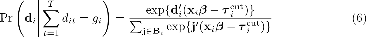
The idea of the BUC-τ estimator is to dichotomize the observations within a person at different cutoff points and then to apply the standard CML estimator. This allows us to estimate the thresholds, too. Let d _i denote the resulting vector of the dichotomized dependent variable for individual i and g_i the number of ones in d _i . In addition, define ${\tau }_i^{\text{cut}}$ as the vector of thresholds used as cutoff points for person i. The conditional probability of observing d _i conditional on g_i , when d _i results from dichotomizing at different cutoff points, is

$\mathrm{Pr}\left(d_i|{\displaystyle \sum _{t=1}^T{d}_{it}=g_i}\right)=\frac{\exp \left\{{d^{\prime }}_i\left(x_i\beta -{\tau }_i^{\text{cut}}\right)\right\}}{{\sum }_{j\in B_i}\exp \left\{j^{\prime }\left(x_i\beta -{\tau }_i^{\text{cut}}\right)\right\}}$

6

where j denotes again a vector with zeros and ones with ${\sum }_{t=1}^T{d}_{it}=g_i$ and B _i the set of all possible j-vectors with g_i ones and T − g_i zeros.

As an example, consider a person who is observed for two time periods. For the BUC estimator, we would produce K − 1 copies of this person’s observations—that is, K − 1 clones of the person—and dichotomize each clone at a different cutoff point. Thus, one of these clones, say, i, would be dichotomized at the cutoff point 3, resulting in $d_i={\left\{1\left(y_i{ }_1\ge 3\right),1\left(y_i{ }_2\ge 3\right)\right\}}^{\prime }$ with corresponding ${\tau }_i^{\text{cut}}=\left({\tau }_3,{\tau }_3\right)\prime$ . The next clone, j, dichotomized at 4, would result in $d_i={\left\{1\left(y_j{ }_1\ge 4\right),1\left(y_j{ }_2\ge 4\right)\right\}}^{\prime }$ with corresponding τ _j ^cut = (τ ₄ , τ ₄)′.

In contrast, for the BUC-τ estimator, the first observation of clone i might be dichotomized at the cutoff point 3 and the second observation at the cutoff point 4, resulting in the vectors $d_i={\left\{1\left(y_i{ }_t\ge 3\right),1\left(y_i{ }_t\ge 4\right)\right\}}^{\prime }$ and ${\tau }_i^{\text{cut}}=\left({\tau }_3,{\tau }_4\right)\prime$ . Thanks to this heterogeneity in the cutoff point within a conditional likelihood contribution (that is, within a clone), the expression depends also on the thresholds, as can be seen in (6).

In the case of the BUC estimator, we combine the (K − 1) possible clones of each person to estimate β . However, if different cutoff points within a clone are allowed as with BUC-τ, the number of possible clones of each person is (K − 1) ^T , and the sample size of the inflated dataset would be N(K − 1) ^T . In standard applications, this would result in more observations than most of today’s computers can handle. Therefore, not all possible clones can be included in the inflated estimation sample, and a selection has to be made. We propose to include all clones with no variation in the cutoff point (that is, the clones corresponding to the sample used by the BUC estimator) and use a limited number of clones with random variation in the cutoff points. The program feologit, threshold is implemented accordingly, where the default is to include 10 clones of each individual with randomly chosen cutoffs. The user can change the number of additional clones by using the option clones(). The process of randomly selecting cutoff points can be influenced by the option seed( # ). With replicability of results in mind, the feologit command has been programmed so that running the BUC-τ estimator twice leads to the same results. This should not deflect from the fact that cutoff points are selected randomly.

3 The feologit estimation command

3.1 Syntax

The command feologit is called with the following syntax:

feologit depvar indepvars [ if ] [ in ] [ weight ], group( varname ) [ thresholds clones( # ) keepsample seed( # ) cluster( clustvar ) or otheropts ]

where depvar is an ordered categorical variable. Time-series operators are not allowed. fweights, iweights, and pweights are allowed (see [U] 11.1.6 weight), but they are interpreted to apply to groups as a whole, not to individual observations.

3.2 Description

feologit fits fixed-effects ordered logit models using the BUC estimator of Baetschmann, Staub, and Winkelmann (2015). It does so by replacing each observation in the dataset by K − 1 copies of the observation (where K is the number of categories of the ordered dependent variable) and then applying the CML estimator clogit, clustering the standard errors at the level of the original panel unit. After estimation, the dataset is returned to its original form (unless the option keepsample is specified). With the option threshold, feologit applies the BUC-τ estimator of Baetschmann (2012), which assumes that thresholds are constant across panel units.

3.3 Options

group( varname ) is required if xtset panelvar has not been specified; it specifies an identifier variable (numeric or string) for the matched groups. If a panel identifier has been set with xtset, the option group( varname ) may be omitted; in this case, feologit will use the panel identifier and provide a warning. strata( varname ) is a synonym for group().

thresholds calls the BUC-τ estimator, which includes estimates of the thresholds.

clones( # ) specifies the number of clones used in the estimation when thresholds has been specified. The default is clones(10). A clone is a copy of all observations of a panel unit.

keepsample specifies that the estimation sample be kept. The estimation sample includes the original data as well as additional observations consisting of copies of the original data. The option keepsample generates the following new variables:

dkdepvar, the dichotomized dependent variable used in the clogit estimation step;

dkthreshold, a variable that indicates at which cutoff point each observation of the ordered dependent variable was dichotomized (to result in dkdepvar);

bucsample, a binary variable that indicates whether the observation forms part of the estimation sample of the BUC estimator—this variable exhibits variation only if the option thresholds has been specified;

clonegroup, an integer-valued variable that identifies observations corresponding to each panel unit and clone in the estimation sample; and

clone, a binary variable that indicates whether an observation is part of the original sample (clone = 0) or a copy (clone = 1).

For instance, after BUC-τ estimation of feologit with the option keepsample, the corresponding BUC estimates can be obtained by issuing the following command:

clogit dkdepvar indepvars if bucsample==1, group(clonegroup) cluster( clustvar )

where indepvars and clustvar are the variables that were used in the BUC-τ estimation.

seed( # ) specifies the pseudo-random-number seed used in the estimation when the option thresholds has been specified. The default is seed(79846512).

cluster( clustvar ) sets the identifier variable for clustering standard errors. Standard errors are always clustered; specifying this option overrides the default clustering variable, which is the group identifier.

or reports the estimated coefficients transformed to odds ratios, that is, exp(b) rather than b. Standard errors and confidence intervals are similarly transformed.

otheropts; see help feologit.

3.4 Stored results

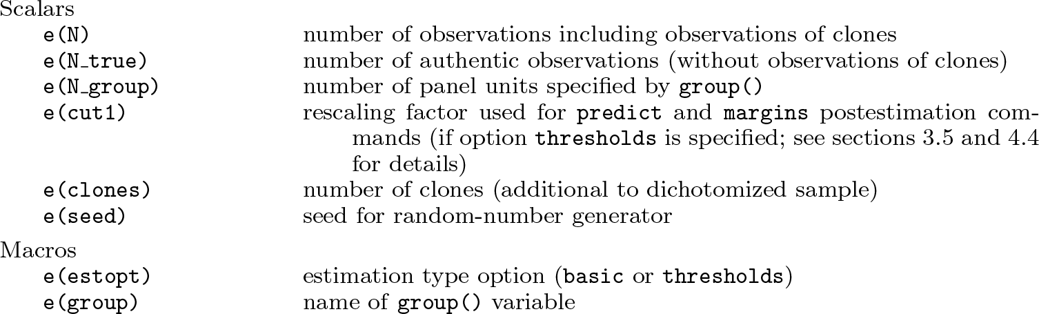
Many of the results stored in e() are similar to clogit or ologit. Stored results specific to feologit are

3.5 Postestimation

The following postestimation commands are available after feologit:

logitmarg calculates statistics of MEs from sample averages. logitmarg uses a routine provided with the feologit installation. It uses sample averages to calculate MEs (see section 4.3 for details). It provides standard errors using the Delta method. The following options allow users to modify the reported results:

– outcome( outcome ) displays estimated MEs only for the category selected by outcome, which should be either one value of the dependent variable or an indicator of the ordered category (#1, #2, etc.).

– dydx( varlist ) displays estimated MEs only for the variables listed by varlist. – eretstore stores estimates in e() instead of r(). Existing e() results will be lost.

predict creates a new variable containing linear predictions (option xb) or predictions of probabilities (called using the same syntax as after ologit). Predictions of probabilities are available only after estimation with the option thresholds. Estimates of probabilities are calculated assuming all fixed effects are equal to e(cut1) (see section 4.4 for details).

margins estimates margins of response for probabilities and linear predictions. Margins for probabilities are available only after estimation with the thresholds option. Margins of response for probabilities are calculated assuming a value of e(cut1) for all fixed effects (see section 4.4 for details).

test and testnl conduct Wald tests of simple and composite linear hypotheses and tests of nonlinear hypotheses. These commands cannot be used on estimates of the second threshold, which is constrained (τ ₂ = 0). The second threshold τ ₂ is the first finite threshold and is called /cut1 in the estimation output.

4 Interpretation

In empirical applications, the interest usually lies in the effect of the covariates x on the dependent variable, and the interpretation of β is of primary interest. However, because the ordered logit model is a nonlinear model, this parameter does not reflect MEs of x on the ordered dependent variable y. There exist different possibilities of interpreting the regression results, some of which are discussed below.

4.1 Direction and compensating variation

The sign of β indicates the direction in which an increase of x influences the cumulative distribution of the dependent variable. If β_l > 0, an increase of the regressor x_l will lead to an unambiguous decrease in the probability of the lowest category Pr(y_it ≥ 1|x _it, α_i ) and an increase in the probability of the highest category Pr(y_it ≥ K|x _it, α_i ). Moreover, the single crossing property of the ordered logit model implies that there will be exactly one change from the probabilities of lower categories, which decrease, to probabilities of higher categories, which increase (see Winkelmann and Boes [2010]). Without knowing the thresholds, one cannot determine at which category this switch from decrease to increase will take place.

The β can be interpreted as MEs of x on the latent variable y ^∗. Because the interest often lies on the ordered dependent variable y rather than the latent y ^∗, this interpretation is rarely used. Another simple interpretation of β with wider application is to compute the compensating variation between variables, for example, the change in two regressors such that the latent variable, and therefore the ordered dependent variable, remains unchanged. The compensating variation of two variables is given by the ratio of the corresponding β : an increase of x_l by 1 has the same effect as an increase of x_r by β_l /β_r .

4.2 Odds ratio

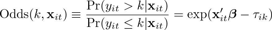
The effect size in logit models is often interpreted using odds, which refers to the ratio between the probability of a certain event and the complementary probability. In the case of ordered logit, the odds of individual i in period t having a y_it above category k relative to below or equal to k is

$\text{Odds}\left(k,x_{it}\right)\equiv \frac{\mathrm{Pr}\left(y_{it}>k|x_{it}\right)}{\mathrm{Pr}\left(y_{it}\le k|x_{it}\right)}=\exp \left({x^{\prime }}_{it}\beta -{\tau }_{ik}\right)$

The odds are independent of the fixed effects but still depend on the thresholds. However, the change in the odds if the lth regressor is modified solely depends on β and the shift of the regressor:

$\text{Odds ratio}\left(k,\Delta x_{itl}\right)\equiv \frac{\text{Odds}\left(k,x_{it}+\Delta x_{itl}\right)}{\text{Odds}\left(k,x_{it}\right)}=\exp \left(\Delta {x^{\prime }}_{itl}\beta \right)$

Therefore, an increase of x_l by 1 increases the odds ratio by exp(β_l ) for all categories except the first one, everything else being equal. Or in other words, a unit increase in x_l changes the odds by about β_l × 100 percent (for small β_l ) or by exactly {exp(β_l ) − 1} × 100 percent. The option or displays the results as exp( β ) as in the standard commands for logit models.

4.3 Marginal effects

In empirical applications, the interest often lies in the marginal probability effects, that is, the change in the probabilities of observing y_it = k if a covariate l is changed by a small amount:

${\text{ME}}_{itkl}=\frac{\partial \mathrm{Pr}\left(y_{it}=k|x_{it},{\alpha }_i\right)}{\partial x_{itl}}=\frac{\partial \mathrm{Pr}\left(y_{it}\le k|x_{it},{\alpha }_i\right)}{\partial x_{itl}}-\frac{\partial \mathrm{Pr}\left(y_{it}\le k-1|x_{it},{\alpha }_i\right)}{\partial x_{itl}}$

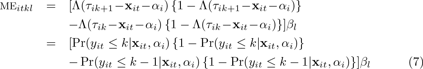
Because the probabilities depend on the thresholds and the individual fixed effects, any marginal probability effects will generally also depend on these parameters. And because they are not estimated, estimates for MEs cannot generally be obtained either. For the ordered logit model, the ME has the specific form

$\begin{array}{c}{\text{ME}}_{itkl}=\left[\Lambda \left({\tau }_{ik}{ }_{+1}-x_{it}-{\alpha }_i\right)\left\{1-\Lambda \left({\tau }_{ik}{ }_{+1}-x_{it}-{\alpha }_i\right)\right\}-\Lambda \left({\tau }_{ik}-x_{it}-{\alpha }_i\right)\left\{1-\Lambda \left({\tau }_{ik}-x_{it}-{\alpha }_i\right)\right\}\right]{\beta }_l\\ =\left[\mathrm{Pr}\left(y_{it}\le k|x_{it},{\alpha }_i\right)\left\{1-\mathrm{Pr}\left(y_{it}\le k|x_{it},{\alpha }_i\right)\right\}-\text{Pr}\left(y_{it}\le k-1|x_{it},{\alpha }_i\right)\left\{1-\mathrm{Pr}\left(y_{it}\le k-1|x_{it},{\alpha }_i\right)\right\}\right]{\beta }_l\end{array}$

7

Thus, we see immediately that the relative size of the MEs of two covariates l and r is equal to the relative size of their β coefficients,

${\text{ME}}_{itkl}{\text{/ME}}_{itkr}={\beta }_l\text{/}{\beta }_r$

a quantity that can readily be estimated from ${\widehat{\beta }}_l\text{/}{\widehat{\beta }}_r$ .

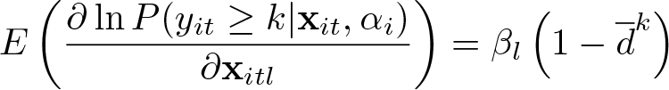
Moreover, from the second equality in (7), it is clear that for given probabilities of the dependent variable y_it , the ME is just a function of β_l and straightforward to calculate with an estimate ${\widehat{\beta }}_l$ . One can therefore calculate MEs for any interesting probabilities of the dependent variable. An obvious choice for such probabilities is the sample proportions. We called this the ME at the average, and it can be computed by the feologit postestimation command logitmarg for each regressor and each possible outcome category. Then, an estimate of the ME of regressor l for category k is

${\overline{\text{ME}}}_{kl}=\left\{{\overline{d}}^{k+1}\left(1-{\overline{d}}^{k+1}\right)-{\overline{d}}^k\left(1-{\overline{d}}^k\right)\right\}{\widehat{\beta }}_l$

where ${\overline{d}}^k$ is the sample average of $d_{it}^k$ . Standard errors for ${\overline{\text{ME}}}_{kl}$ can be obtained via the Delta method. Depending on whether one is interested in ${\overline{\text{ME}}}_{kl}$ as an estimate of the ME at the sample average or as an estimate of the ME at the population mean, standard errors need to account for sampling variation from estimation of only β or, in addition, from estimation in ${\overline{d}}^{k+1}$ and ${\overline{d}}^k$ . The command logitmarg provides standard errors for the ME at the sample average.

This is a simple and arguably useful object of interest. However, it is different from the average ME, E(ME _itkl ), which is infeasible. It is also different from the ME at the average of the regressors, defined as (7) evaluated at $\overline{x}={\sum }_i{\sum }_t{x}_{it}\text{/}\left(NT\right)$ , which is also infeasible. Both of these more widely used objects of interest depend on the unavailable individual thresholds and fixed effects [see the expression after the first equality of (7)], while the ME at the average of the dependent variable that we propose circumvents this problem by focusing instead on the expression after the second equality of (7).

Finally, another potentially useful quantity that is identified and easily estimable is the average semielasticity of the continuation probability at category k with respect to regressor l. The identification and estimation of the average semielasticity in binary fixed-effects logit models was demonstrated by Kitazawa (2012) (see also Santos Silva and Kemp [2016]), and here we generalize it to the ordered case:

$E\left(\frac{\partial \ln P\left(y_{it}\ge k|x_{it},{\alpha }_i\right)}{\partial x_{itl}}\right)={\beta }_l\left(1-{\overline{d}}^k\right)$

4.4 Thresholds

The assumption of constant thresholds for all individuals used by the BUC-τ estimator allows for additional interpretations. A model with constant thresholds can be fit with feologit by using the option threshold. For the interpretations that follow, we change our conceptual perspective: up to this point, all interpretations were cast in terms of probabilities. The ε_it was treated as a random variable. Now, we keep ε_it fixed, and a change of a regressor leads to a deterministic effect of either pushing the ordered variable to a different category or staying in the same category.

If the spaces between adjacent thresholds are almost equal, a change of the regressors has similar effects independently of the specific category. This does not apply, however, for the tails of the distribution, that is, the lowest and the highest category. If the spaces are unequal, a change of a regressor has a smaller effect for categories where the thresholds are far apart.

Regarding the effects of covariates, even a marginal change can lead to a switch of category because we do not know the exact value of the latent variable. However, because an estimate of the differences between the thresholds is available, we can also compute the change in the regressors, which surely leads to a switch of category. For example, a person in the third category will surely rise up to the next higher category if x _itl increases by (τ ₃ − τ ₄)/β_l , everything else being equal.

When both the thresholds and β are known, the only unknown parameter in the formula for the ME (7) is α_i . For such situations in fixed-effects models, Stata’s margins postestimation command assumes α_i = 0 for all i. This is the case, for instance, when using margins after xtlogit with the option fe (the binary fixed-effects logit).

If α_i ≠ 0 for all i, the object estimated assuming α_i = 0 for all i will, in general, not be consistent for the average ME. Nevertheless, we have equipped feologit with a similar postestimation capability. When margins is called after feologit with the option thresholds, an average ME is computed assuming that α_i is constant across individuals. Because of the underidentification of τ_ik and α_i , and the normalization τ ₂ = 0, calculating probabilities at α_i = 0 for all i is often a particularly poor choice. Therefore, we use ${\alpha }_i=\tilde{\alpha }$ for all i instead, which is defined as the estimate of the constant in a binary (cross-sectional) logit of the dichotomized dependent variable at the first cutoff $\left(d_{it}^2\right)$ with a single regressor $z_{it}\equiv x_{it}\widehat{\beta }$ whose coefficient is restricted to 1:

$\tilde{\alpha }=\underset{a}{\max }{\displaystyle \sum _i{\displaystyle \sum _t{d}_{it}^2\log \Lambda \left(a+z_{it}\right)+\left(1-d_{it}^2\right)}}\left\{1-\Lambda \left(a+z_{it}\right)\right\}$

with first-order condition

${\overline{d}}^2={\left(NT\right)}^{-1}{\displaystyle \sum _i{\displaystyle \sum _t\Lambda \left(\tilde{\alpha }+z_{it}\right)}}$

The estimate $\tilde{\alpha }$ is stored in e(cut1) after feologit with the option thresholds. A potentially better estimate for $\tilde{\alpha }$ could be obtained by using all d^k instead of basing it only on d ². However, our intention here is to provide such an estimate only as a suggestive result, and we caution against relying on these MEs (see also, for example, Santos Silva and Kemp [2016], who argue persuasively against using MEs based on α_i =0).

5 Application: Effect of motherhood on life satisfaction

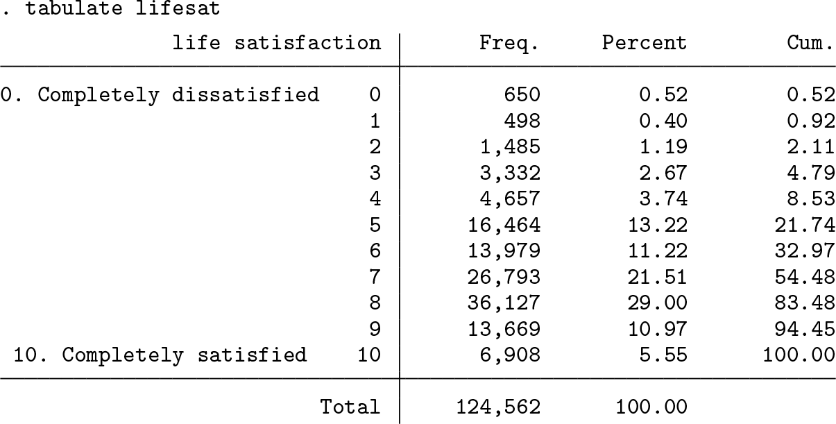
To illustrate the empirical application of the feologit command, we analyze the effect of the birth of the first child on his or her mother’s life satisfaction using the SOEP, a large representative household survey (Wagner, Frick, and Schupp 2007). The data were collected yearly between 1984 and 2009, and it is therefore possible to follow a person up to 26 years. The sample includes women between the ages of 20 and 60 who either were mothers or became mothers during the observation period. The application is based on data from Baetschmann, Staub, and Studer (2016), where additional information about data and estimation of causal effects can be found. ² The dependent variable is life satisfaction, an ordinal variable that ranges from 0 (completely dissatisfied) to 10 (completely satisfied). Below, we tabulate its distribution.

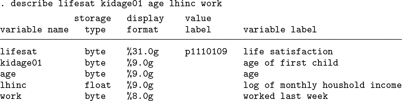
About two-thirds of the responses lie in the upper part of the distribution (seven or higher). The modal answer is category 8 with a proportion of around 29%. We want to analyze the effect of the first child on a mother’s life satisfaction and are especially interested in the evolution of a woman’s general life satisfaction in the first years after the birth of her first child. Our specification also includes a small set of additional regressors: age, logarithm of household income, and a dummy indicating whether the respondent is working. While controlling for potentially endogenous factors such as income and labor-force participation can lead to biases in the estimates of the effects of interest, we include these variables here only to illustrate the regression output of the feologit command.

To estimate the effect of having the first child on life satisfaction and the following dynamics, we include five dummy variables, representing the age of the first child in years. For example, the variable kidage01_2 is equal to 1 when the first child’s age is 2 and 0 otherwise. Such a flexible form approach is common in the literature on adaptation to life events (for example, Clark et al. [2008]). Women who are happier might be more likely to get married and have children (Stutzer and Frey 2006). To control for this selection into motherhood, we want to control for time-invariant characteristics like a genetic disposition to happiness. And because the dependent variable is ordered, we use a fixed-effects ordered logit model fit with the BUC estimator. First, we declare the panel variable with the xtset command,

. xtset idpers

panel variable: idpers (unbalanced)

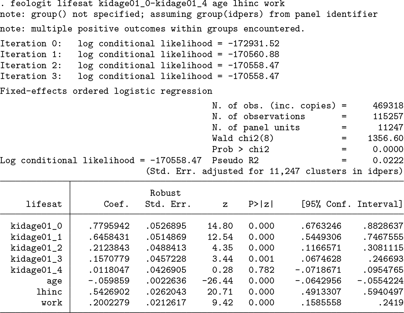
and then fit the model with the BUC estimator using feologit. We issued the following command:

The output shows that the algorithm for maximizing the log conditional likelihood converged after three steps. For fitting the model parameters, only individuals (panel units) who have variation in their dependent variables are informative. Individuals who are observed only once or have always the same life satisfaction scores over time are excluded by the program (because their LL contribution is zero). This condition is met by 11,247 individuals, which results in 115,257 observations. On average, people in the estimation sample are therefore observed about 10 times. The ordered dependent variable has 11 categories, so 10 different dichotomizations are possible. However, because not all dichotomizations lead to copies with variation in the binary dependent variable, we end up with 469,318 copies that contribute to the estimation procedure. Because the copies are not independent of each other, feologit calculates cluster-adjusted standard errors at the individual level (11,247 individuals).

The Wald test indicates that all eight included variables are jointly statistically significant. Regarding the effect of having the first child, the effect is highest in the year of birth (coefficient on kidage01_0). Thereafter, the effect decreases and reaches a nonsignificant level after four years. Age has a negative effect after controlling for timeinvariant characteristics and the other variables in the model. As expected, household income and working have a positive effect on life satisfaction. The compensating variation between work and log household income is about 0.37, meaning that log household income has to increase by 0.37 to compensate for not working. This is equivalent to saying that household income has to increase by 45% [exp(0.37)−1] to offset a nonworking status.

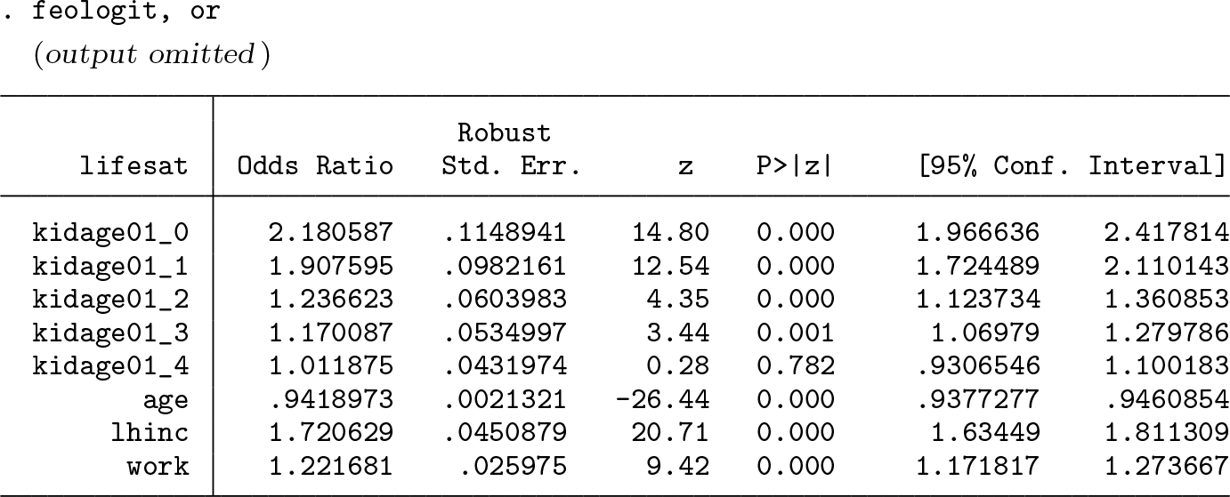
Odds ratios for interpreting the effect sizes can be obtained by using the option or. Below are the code and an excerpt of the output:

Having the first child increases the odds ratio by about 118% in the year of birth, about 91% in the first, about 24% in the second, and about 17% in the third year thereafter. In the fourth year, the effect is essentially no longer present.

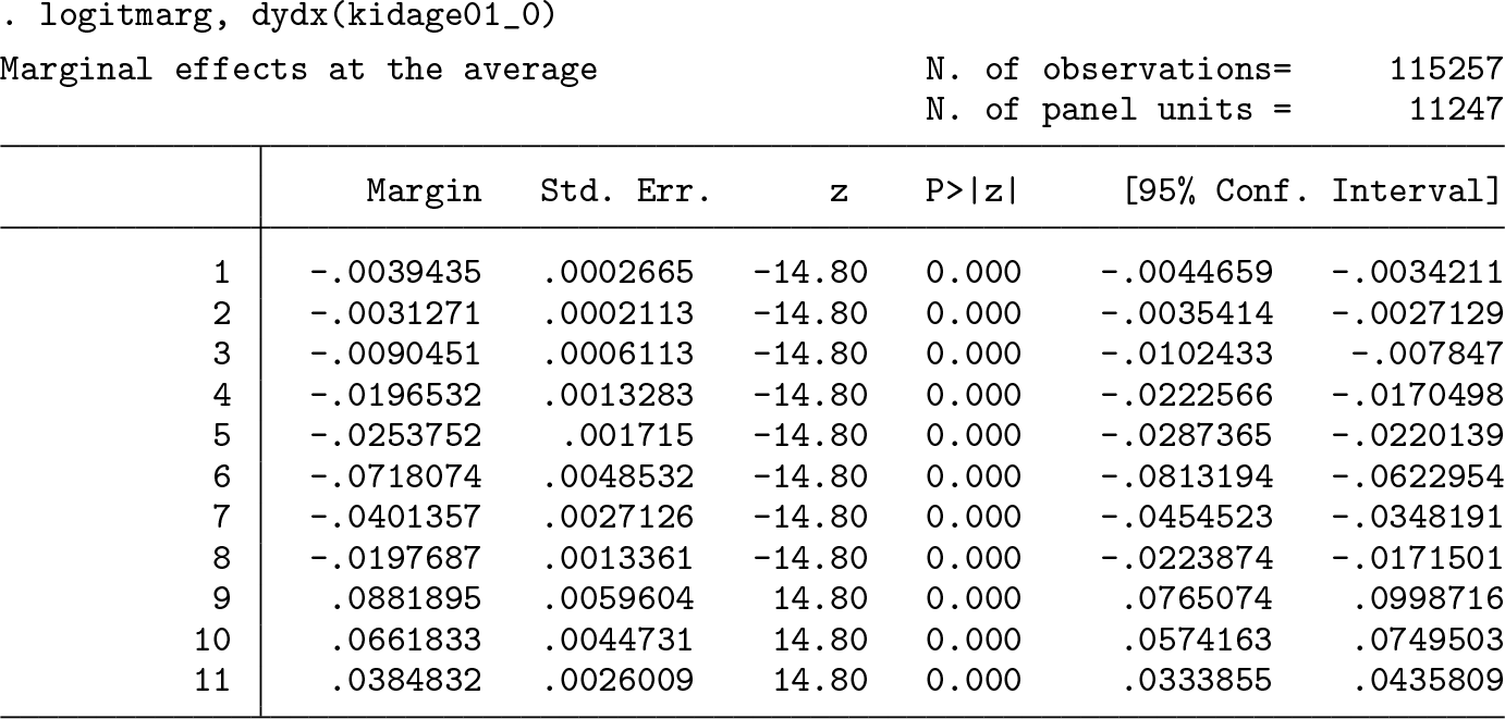
Marginal effects at the average can be obtained by using the postestimation command logitmarg after fitting the model. They are computed using the relative frequencies of the corresponding categories in the estimation sample. Below are the code and the output. We specified the option dydx(kidage01_0) to limit the output to the MEs of the year of birth.

Note that logitmarg enumerates categories starting at 1 and ignores the actual (arbitrary) labels of the dependent variable, which in our case starts at 0. Because having a child has a positive effect on life satisfaction in the first year, the marginal probability effects at the average are negative for the lower categories and positive for the ninth and higher categories. For example, in the first year having a child decreases the probability of falling into the sixth category by 7.2% points and increases the probability of having the highest rating by 3.8% points for this average person, everything else being equal. The effects for the lowest categories are small because only a few people have such a low life-satisfaction status.

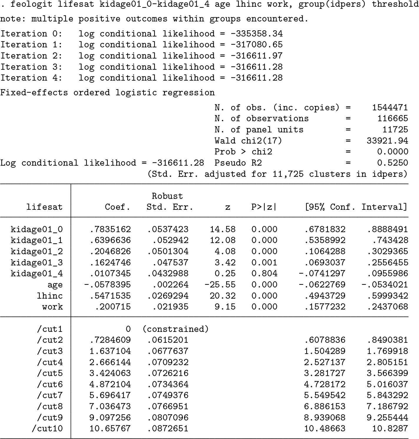
Estimating the thresholds is possible by using the option thresholds, which calls the BUC-τ estimator. This requires the assumption that the spacing between the thresholds is the same for all individuals. Below is the output:

In contrast with the procedure without thresholds, the cutoff point within a likelihood contribution (clone) can change. Therefore, even when the ordered dependent variable is constant, the resulting dichotomized dependent variable with different cutoff points can vary. This increases the number of individuals in the estimation sample slightly to 11,725 and the number of observations to 116,665. The estimator includes all contributions of the BUC estimator plus 10 copies of each individual with random variation in the cutoff point. Therefore, the number of included copies increases noticeably to over 1.5 million.

The regression coefficient β has the same interpretation as before. One can also display the odds ratios. From the output, we see that the exact estimates changed only slightly. Because life satisfaction can take 11 different values and the first finite threshold /cut1 (corresponding to τ ₂) is normalized to zero, the output shows estimates for the 2nd to the 10th threshold. Careful inspection of the spaces shows that there is a moderate tendency that differences increase toward the top. Where the difference between the first and second, and second and third, is 0.728 and 0.909, respectively, the two spaces at the upper end are 2.06 and 1.56. This implies that changes of regressors have a larger effect on the observed ordered dependent variable for unhappy individuals compared with happy individuals.

The spaces range from 0.73 to 2.06, where the second smallest difference is 0.76. The size of the MEs of the different regressors are rather small compared with these spaces. Except for the unhappiest people (lowest category), having a child can never increase life satisfaction by more than one point, everything else being equal. The same is true for doubling the income [exp(0.547) = 1.73]. Regarding age, for a person with a life satisfaction score of 9, 26 years need to pass for her to surely change to the next lower category [(10.35 − 8.91)/0.057].

The BUC and BUC-τ estimator are both consistent under the additional assumption of constant thresholds. Therefore, we can test this assumption in the form of a generalized Hausman specification test by comparing the two estimates. If they are statistically different, we can reject the null hypothesis of constant thresholds. ³ There are different possibilities to implement such a test in Stata. The most obvious way would be to use the command suest. Using this command requires fitting the model without clustered standard errors and, in a second step, computing a joint covariance matrix of both estimators adjusting for clusters. However, because computing the BUC estimator without clusters can be misleading and adjusting them after using clogit can lead to error messages if the group variable is not properly nested within the cluster variable, we decided to work with interaction terms. In a first step, the command feologit, threshold with the additional option keepsample is used:

. quietly: feologit lifesat kidage01_0-kidage01_4 age lhinc work, group(idpers) > threshold keep

The option keepsample, here shortened to keep, keeps the inflated dataset of clones that is used to compute the BUC-τ estimator after the estimation. In addition, the dichotomized dependent variable is stored under dkdepvar, the corresponding cutoff point under dkthreshold, and the variable bucsample indicates whether the cutoff varies within the clone (bucsample = 0) or not (bucsample = 1). Observations with bucsample = 1 constitute the sample of the BUC estimator. The remaining observations are primarily used to estimate the thresholds but contribute to the estimates of β , too. Under the null hypothesis of constant thresholds, both samples (bucsample = 0 and bucsample = 1) can be used to estimate β . Statistical differences between the two estimates indicate that the thresholds are not constant. Thus, after having used feologit with the options thresholds and keepsample, we can implement this test by interacting the variable bucsample with all regressors and fitting the model with clogit while grouping on the clone variable and clustering on the individual level. Finally, we test whether the differences of the interaction terms are jointly equal to zero.

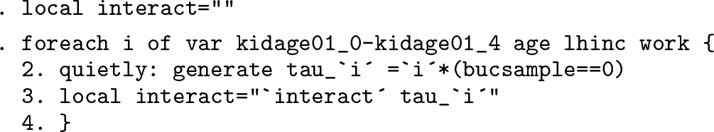
As an auxiliary step, we first use a small loop to create the interaction variables (prefixed tau_ ) and store them in the local macro interact:

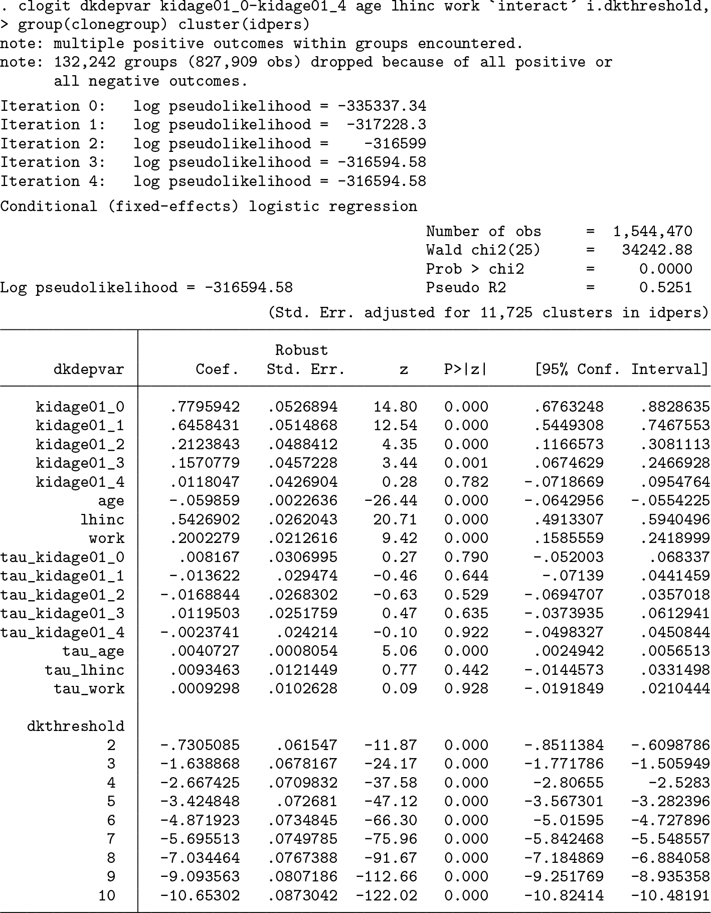
We then fit the model with interactions using the clogit command, grouping on the clone variable and clustering on the individual level:

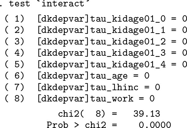
As can be seen, the estimates of the noninteracted regressors are numerically equivalent to the previous BUC estimates. The estimates of the interaction terms mirror the differences between the BUC and the BUC-τ estimates but are not identical because the thresholds adjust to the additional regressors. The differences are small, and most of them are not individually significant. To formally test whether they are jointly different, we can use Stata’s test command:

Despite the differences being small, the joint hypothesis that all these terms are equal to zero can be rejected at the 0.1% level [χ ²(8) = 39.13] because of the large sample. Therefore, formally we reject the null hypothesis of constant thresholds and should use the BUC instead of the BUC-τ estimator to interpret the results. However, given that differences in the estimates in this case are so small, the thresholds might still shed some light on the data-generating process but should not be overinterpreted.

6 Conclusion

In this article, we presented and discussed the BUC and BUC-τ estimators of the fixedeffects ordered logit model and introduced a new community-contributed command that implements these estimators in Stata, feologit.

BUC and BUC-τ both offer consistent estimates of the slope parameters β . In addition, BUC-τ obtains consistent estimates of the thresholds τ, under the slightly more restrictive assumption that they do not vary between individuals. While the calculation of average MEs is not possible with these estimators, useful identified objects of interest include odds ratios, compensating variation, and other quantities. Of particular interest is a particular ME at the average, which we proposed in this article and for which a dedicated postestimation command is available with feologit. Finally, we also presented a new specification test that can be used to evaluate the assumption of constant thresholds by comparing BUC and BUC-τ estimates and that can be easily implemented with a few lines of code in Stata.

8 Programs and supplemental materials

Supplemental Material, st0596 - feologit: A new command for fitting fixed-effects ordered logit models

Supplemental Material, st0596 for feologit: A new command for fitting fixed-effects ordered logit models by Gregori Baetschmann, Alexander Ballantyne, Kevin E. Staub and Rainer Winkelmann in The Stata Journal