Sage Journals: Discover world-class research

Abstract

When one analyzes the determinants of production efficiency, regressing efficiency scores estimated by data envelopment analysis on explanatory variables has much intuitive appeal. Simar and Wilson (2007, Journal of Econometrics 136: 31–64) show that this conventional two-stage estimation procedure suffers from severe flaws that render its results, and particularly statistical inference based on them, questionable. They additionally propose a statistically grounded bootstrap-based two-stage estimator that eliminates the above-mentioned weaknesses of its conventional predecessors and comes in two variants. In this article, we introduce the new command simarwilson, which implements either variant of the suggested estimator in Stata. The command allows for various options and extends the original procedure in some respects. For instance, it allows for analyzing both outputand input-oriented efficiency. To demonstrate the capabilities of simarwilson, we use data from the Penn World Tables and the Global Competitiveness Report by the World Economic Forum to perform a cross-country empirical study about the importance of quality of governance in a country for its efficiency of output production.

Keywords

st0585 simarwilson simarwilson postestimation gciget Global Competitiveness Index DEA two-stage estimation truncated regression bootstrap efficiency bias correction environmental variables

1 Introduction

Analyzing the technical efficiency of production or decision-making units (DMUs) has developed into a major field in empirical economics and management science.¹ From a methodological perspective, the two most popular strands of the literature can be distinguished: i) analyses that rest on parametric, regression-based methods, namely, stochastic frontier analysis (Aigner, Lovell, and Schmidt 1977), and ii) analyses that use nonparametric methods, namely, data envelopment analysis (DEA) (Charnes, Cooper, and Rhodes 1978). The pros and cons of either approach have been discussed extensively (for example, Hjalmarsson, Kumbhakar, and Heshmati [1996]; Murillo-Zamorano [2004]).

One of the advantages of the parametric approaches, namely, the truncated normal stochastic frontier model, is that it not only allows for measuring inefficiency but also incorporates a model of the determinants of inefficiency.² In contrast, nonparametric approaches are primarily concerned with estimating a production-possibility frontier (or an input-requirement frontier) and with measuring the distance of observed input-output combinations to this frontier. However, shedding light on what determines the magnitude of this distance is out of the narrow³ scope of nonparametric approaches such as DEA.

For many research questions, however, identifying determinants of inefficiency is more relevant than determining its magnitude for specific DMUs. For this reason, in the domain of nonparametric efficiency analysis, semiparametric two-stage approaches that combine efficiency measurement by DEA with a regression analysis that uses DEA estimated efficiency as dependent variables have become popular. Simar and Wilson (2007) list almost 50 published articles and mention hundreds of unpublished articles that use such two-stage procedures. In these (early) applications, the second stage is typically a censored (tobitlike) regression to account for the bounded nature of DEA efficiency scores or just simply ordinary least squares (Simar and Wilson 2007).

Despite their popularity and their intuitive appeal, such conventional two-stage estimators are criticized by Simar and Wilson (2007) mainly for two reasons. First, they stress the absence of a clear theory of the underlying data-generating process that would justify the conventional two-stage approach.⁴ Second, they criticize the conventional inference that is pursued in most two-stage applications for ignoring that estimated DEA efficiency scores are calculated from a common sample of data. Treating them as if they were independent observations is not appropriate, because the problems related to invalid inference due to serial correlation arise. Simar and Wilson (2007) develop a two-stage procedure that accounts for the above-mentioned issues. They describe an underlying data-generating process that is consistent with a two-stage estimation procedure, which—as the most obvious difference to the earlier conventional approach—implies a truncated rather than censored regression model. This reflects that the substantial share of fully efficient DMUs typically found in DEA is an artifact of the finite-sample bias inherent in DEA but does not represent a feature of the true underlying data-generating process. Moreover, they propose two parametric bootstrap procedures that are consistent with the assumed data-generating process and address the second issue. They yield estimated standard errors and confidence intervals that do not suffer from bias due to estimated efficiency scores being correlated.

The Simar and Wilson (2007) procedure has become a workhorse of empirical efficiency analysis with hundreds of applications from various fields of economics.⁵ This popular, but technically involved estimator, has not yet been available to Stata users unless they developed their own code. In this article, we introduce the new command simarwilson, which allows for applying this estimator in Stata.⁶ In doing this, it greatly benefits from the recently published community-contributed command teradial (Badunenko and Mozharovskyi 2016), which is required for running simarwilson. For the first time, teradial enables fast estimation of DEA in Stata even for large samples. This is essential for practical applications of the Simar and Wilson (2007) estimator because it involves bootstrapping the DEA estimator.⁷

The remainder of this article is organized as follows. Section 2 gives a brief summary of the Simar and Wilson (2007) two-stage estimator. Section 3 describes the syntax of simarwilson. Section 4 presents an application to cross-country data. Section 5 concludes.

2 The Simar and Wilson (2007) estimator in brief

2.1 Some essential ideas

Simar and Wilson (2007) consider a setting in which a researcher observes three types of variables x _i, y _i, and z _i for a sample of $i = 1, . . ., N$ DMUs. x _i denotes a vector of P inputs to production. y _i is a vector of Q outputs from production. z _i denotes a row vector of K environmental variables that may affect the ability of DMU i to efficiently combine the consumed inputs to the produced outputs. The effect of z _i on efficiency is in the focus of the empirical analysis. The production technology is assumed to be homogeneous across DMUs. That is, a common production-possibility frontier—the boundary of the convex production-possibility set—represents all combinations $(y_{j}^{^{*}}, x_{j}^{^{*}})$ that are fully efficient in that no output can be increased without decreasing at least one other output or increasing at least one input (Koopmans 1951). A crucial assumption is that the shape of the production-possibility frontier does not depend on z _i, which is referred to as separability in Simar and Wilson (2007).

The output-input set (y _i, x _i) observed for DMU i will regularly fail in realizing a point at the frontier. This deviation is necessarily directional; that is, i produces less output than technically feasible, or it consumes more input than technically feasible. The widely used output-oriented Farrell (1957) distance measure quantifies the deviation from the frontier as the relative radial distance in output direction θ _i. That is, θ _i denotes the factor by which output generation y _i of DMU i has to be proportionally increased to project (y _i, x _i) onto the frontier. θ _i is hence a measure of inefficiency that is bounded to the [1, ∞) interval. Alternatively, one may measure the Farrell distance in input direction as ϑ _i, that is, the factor by which input consumption x _i of DMU i has to be proportionally reduced to project (y _i, x _i) onto the frontier. Hence, ϑ _i is a measure of efficiency that is bounded to the (0, 1] interval.⁸ Yet, in Simar and Wilson (2007), the focus is on θ _i.⁹

The key idea in Simar and Wilson (2007) about the data-generating process is that efficiency θ _i linearly depends on z _i,

θ_{i} = z_{i} β + ε_{i}

where β denotes a column vector of coefficients, the estimation of which is the ultimate objective of the empirical analysis. The disturbances ε _i are assumed to be statistically independent across DMUs¹⁰ and to follow a truncated normal distribution with parameters $µ = 0$ and σ and left-truncation at $1 - z_{i} β$ .¹¹ This assumption guarantees that θ _i cannot be smaller than unity irrespective of the values the variables in z _i may take. Though full efficiency $(θ_{i} = 1)$ is in principle possible, it occurs with zero probability. Conditional on θ _i, DMU i chooses a set of outputs and inputs $(y_{i}, x_{i})$ as $(y_{i}^{*} / θ_{i}, X_{i}^{*})$ , with $(y_{i}^{*}, X_{i}^{*})$ denoting some point on the production-possibility frontier.¹² That is, rather than the technically feasible amount of output $y_{i}^{*}$ , only $(100 / θ_{i})$ percent of $y_{i}^{*}$ is actually produced.

It is key for understanding the shortcomings of conventional two-stage approaches that θ _i is genuinely unobservable. Consequently, the estimated efficiency score ${\hat{θ}}_{i}$ , which is obtained by running a DEA,¹³ is not θ _i. In other words, ${\hat{θ}}_{i}$ is not the distance of $(y_{i}, x_{i})$ to the true production-possibility frontier, but the distance to an estimate of the latter. Because of the boundary estimation framework of DEA, this estimate suffers from finite-sample bias, and in turn ${\hat{θ}}_{i}$ is biased toward the value of 1. That means that (1) cannot be estimated straightforwardly, and θ _i has to be replaced in (1) by the biased estimate ${\hat{θ}}_{i}$ to formulate an operational regression equation. As pointed out in Simar and Wilson (2007), this generates two major problems for conventional two-step approaches. First, although the errors ε _i are assumed to be statistically independent across DMUs, the operational errors in a regression of ${\hat{θ}}_{i}$ on z _i are not, because the ${\hat{θ}}_{i}$ are estimated from a common sample of data. Second, in any application of DEA some—usually numerous— ${\hat{θ}}_{i}$ take the value of 1, though according to (1), θ _i takes this value with zero probability.

In the procedure¹⁴ suggested in Simar and Wilson (2007), the former issue is addressed by estimating standard errors and confidence intervals for $\hat{β}$ with a parametric bootstrap procedure, in which artificial pseudoerrors are independently drawn from the truncated normal distribution with left-truncation at $1 - z_{i} \hat{β}$ . The latter issue is addressed in Simar and Wilson (2007) in two ways, which leads to two different suggested estimation procedures (algorithm 1 and algorithm 2). Algorithm 1 simply excludes those DMUs from the regression analysis, for which DEA yields scores ${\hat{θ}}_{i}$ that equal 1. These are obviously artifacts of finite-sample bias. The remaining M (with M < N) DEA scores enter a truncated regression model (left-truncation at 1) as the left-handside variable. Fitting this model yields $\hat{β}$ , which, together with the estimate for the variance parameter $\hat{σ}$ , enters the bootstrap procedure mentioned above. The second suggested approach (algorithm 2) is more involved and rests on bias-corrected DEA scores ${\hat{θ}}_{i}^{b c}$ as the left-hand-side variable. Because ${\hat{θ}}_{i}^{b c} > 1$ holds for $i = 1, . . ., N$ , unlike algorithm 1, all DMUs are considered in the truncated regression analysis and the subsequent bootstrap procedure. The bias correction itself rests on a bootstrap procedure that incorporates the assumptions regarding the data-generating process of θ _i, that is, (1). For this reason, it is computationally simpler and more parametric than alternative bias-correction procedures that have been suggested in the literature (Simar and Wilson 2000; Kneip, Simar, and Wilson 2008) and have recently been made available to Stata users by the community-contributed command teradialbc (Badunenko and Mozharovskyi 2016).

Figure 1 graphically illustrates (and the notes below describe) the concepts of true, DEA estimated, and bias-corrected estimated inefficiency, using randomly generated data and considering a simple single input–single output production technology.

Figure 1.

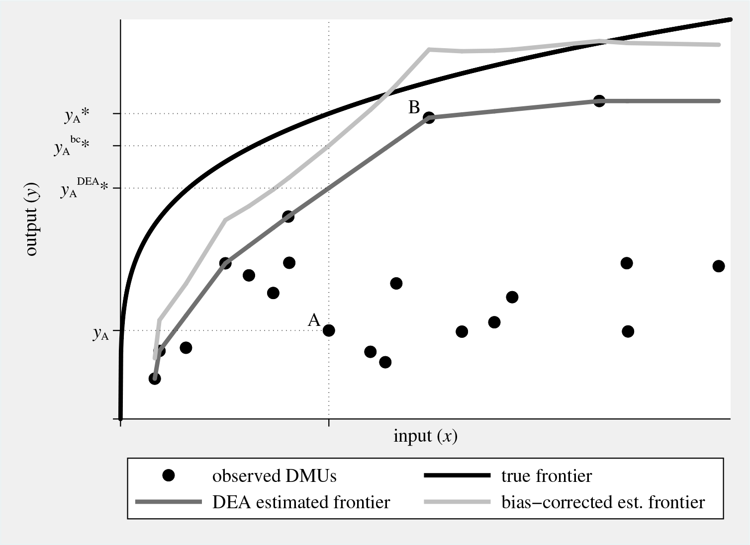
Graphical illustration of true and estimated inefficiency. Considering DMU A, true inefficiency θ _A is $y_{A}^{*} / y_{A}$ , (uncorrected) DEA estimated inefficiency ${\hat{θ}}_{A}$ is $y_{A}^{D E A *} / y_{A}$ , and bias-corrected estimated inefficiency ${\hat{θ}}_{A}^{b c}$ is $y_{A}^{^{b c *}} / y_{A}$ . In this finite and small (N = 20) artificial sample, DEA systematically underestimates true inefficiency. Bias correction adjusts estimated inefficiency upward. DMU B, for instance, which is seemingly fully efficient according to conventional DEA, is inefficient according to the biascorrected estimated frontier. Indeed, the inefficiency of B is even overestimated by ${\hat{θ}}_{B}^{b c}$ . Unlike for conventional DEA, with bias correction the estimated production-possibility set is not convex; the estimated frontier is not even monotone. NOTE: Input quantities x randomly drawn from continuous uniform U(0, 2) distribution; true frontier (production function) $y = x^{1 / 4}$ ; inefficiency generated according to (1), with $β = 0$ and $σ = 3$ ; variable returns to scale assumed in the DEA; bias correction follows steps 1–4, algorithm 2 (Simar and Wilson [2007]; see below). SOURCE: Calculations are our own.

2.2 The procedures suggested in Simar and Wilson (2007)

This subsection describes in detail the suggested procedures algorithm 1 and algorithm 2. In doing this, it almost exactly reproduces what is found on pages 41–43 in Simar and Wilson (2007). This particularly applies to the subsequent numbered paragraphs that describe the steps of the estimation procedures almost exactly as they are described in the key reference.

Algorithm 1 consists of the following steps:

1. Compute ${\hat{θ}}_{i}$ for all DMUs $i = 1, . . ., N$ using DEA.

2. Use those M (with M < N) DMUs for which ${\hat{θ}}_{i} > 1$ holds in a truncated regression (left-truncation at 1) of ${\hat{θ}}_{i}$ on z _i to obtain coefficient estimates $\hat{β}$ and an estimate for variance parameter $\hat{σ}$ by maximum likelihood.

3. Loop over the following steps 3.1–3.3 B times to obtain a set of B bootstrap estimates $({\hat{β}}^{b}, {\hat{σ}}^{b})$ , with $b = 1, . . ., B .$

3.1. For each DMU $i = 1, . . ., M$ , draw an artificial error ${\tilde{ε}}_{i}$ from the truncated $N (0, \hat{σ})$ distribution with left-truncation at $1 - z_{i} \hat{β}$ .

3.2. Calculate artificial efficiency scores ${\hat{θ}}_{i}$ as $z_{i} \hat{β} + {\tilde{ε}}_{i}$ for each DMU $i = 1, . . ., M$ .

3.3. Run a truncated regression (left-truncation at 1) of ${\hat{θ}}_{i}$ on z _i to obtain maximum-likelihood bootstrap estimates ${\hat{β}}^{b}$ and ${\hat{σ}}^{b}$ .

4. Calculate confidence intervals and standard errors for $\hat{β}$ and $\hat{σ}$ from the bootstrap distributions of ${\hat{β}}^{b}$ and ${\hat{σ}}^{b}$ .

The more involved algorithm 2 consists of the following steps:

1. Compute ${\hat{θ}}_{i}$ for all DMUs $i = 1, . . ., N$ using DEA.

2. Use those M (M < N) DMUs for which ${\hat{θ}}_{i} > 1$ holds in a truncated regression (left-truncation at 1) of ${\hat{θ}}_{i}$ on z _i to obtain coefficient estimates $\hat{β}$ and an estimate for variance parameter $\hat{σ}$ by maximum likelihood.

3. Loop over the following steps 3.1–3.4 B ₁ times to obtain a set of B ₁ bootstrap estimates ${\hat{θ}}_{i}^{b}$ for each DMU $i = 1, . . ., N$ , with $b = 1, . . ., B_{1}$ .

3.1. For each DMU $i = 1, . . ., N$ , draw an artificial error εe_i from the truncated $N (0, \hat{σ})$ distribution with left-truncation at $1 - z_{i} \hat{β}$ .

3.2. Calculate artificial efficiency scores ${\hat{θ}}_{i}$ as $z_{i} \hat{β} + \tilde{ε}$ for each DMU $i = 1, . . ., N$ .

3.3. Generate $i = 1, . . ., N$ artificial DMUs with input quantities ${\tilde{x}}_{i} = x_{i}$ and output quantities ${\tilde{y}}_{i} = ({\hat{θ}}_{i} / {\tilde{θ}}_{i}) y_{i}$ .

3.4. Use the N artificial DMUs, generated in step 3.3, as reference set in a DEA that yields ${\hat{θ}}_{i}^{b}$ for each original DMU $i = 1, . . ., N$ .

4. For each DMU $i = 1, . . ., N$ , calculate a bias-corrected efficiency score ${\hat{θ}}_{i}^{b c}$ as ${\hat{θ}}_{i} - {(1 / B_{1}) \sum_{b = 1}^{B_{1}} {\hat{θ}}_{i}^{b} - {\hat{θ}}_{i}}$ .

5. Run a truncated regression (left-truncation at 1) of ${\hat{θ}}_{i}^{b c}$ on z _i to obtain coefficient estimates $\hat{\hat{β}}$ and an estimate for variance parameter $\hat{\hat{σ}}$ by maximum likelihood.

6. Loop over the following steps 6.1–6.3 B ₂ times to obtain a set of B ₂ bootstrap estimates ( ${\hat{\hat{β}}}^{b}$ , ${\hat{\hat{σ}}}^{b}$ ), with $b = 1, . . ., B_{2}$ .

6.1. For each DMU $i = 1, . . ., N$ , draw an artificial error ${\hat{\hat{ε}}}_{i}$ from the truncated $N (0, \hat{\hat{σ}})$ distribution with left-truncation at $1 - z_{i} \hat{\hat{β}}$ .

6.2. Calculate artificial efficiency scores ${\tilde{\tilde{θ}}}_{i}$ as $z_{i} \hat{\hat{β}} + {\hat{\hat{ε}}}_{i}$ for each DMU $i = 1, . . ., N$ .

6.3. Run a truncated regression (left-truncation at 1) of ${\tilde{\tilde{θ}}}_{i}$ on z _i to obtain bootstrap estimates ${\hat{\hat{β}}}^{b}$ and ${\hat{\hat{σ}}}^{b}$ by maximum likelihood.

7. Calculate confidence intervals and standard errors for $\hat{\hat{β}}$ and $\hat{\hat{σ}}$ from the bootstrap distribution of ${\hat{\hat{β}}}^{b}$ and ${\hat{\hat{σ}}}^{b}$ .

simarwilson uses the inverse-transform method for generating pseudotruncated normal random variates.¹⁵ Choosing sufficiently large values for B ₁ and B ₂—the latter corresponds to B in algorithm 1—is crucial for the bias correction and estimation of percentile-based confidence intervals yielding meaningful results. For B ₁ and B ₂, simarwilson uses the default of 100 and 1,000 bootstrap repetitions, respectively. The former default value is suggested in Simar and Wilson (2007), yet depending on the data used, choosing a substantially larger number for B ₁ may be advisable. If normal-approximated confidence intervals (option cinormal) are preferred, one may choose a much smaller number than the default for B and B ₂, respectively. Running simarwilson, particularly algorithm 2, requires a substantial amount of computing time, which rapidly increases in the number of observations and the number of inputs and outputs in DEA. For small samples, looping over truncated regression takes the lion’s share of computing time. If the sample is large, looping over DEA consumes relatively more time.¹⁶

2.3 Some minor extensions

The new command simarwilson is meant to implement the above procedures one to one in Stata. It deviates from what is suggested in Simar and Wilson (2007) only by allowing for some settings and features that are not explicitly considered there.

simarwilson allows for analyzing input-oriented efficiency, while Simar and Wilson (2007) consider only the output-oriented counterpart. This requires estimating an input-oriented efficiency measure ${\hat{ϑ}}_{i}$ in step 1 (algorithm 1) and steps 1 and 3.4 (algorithm 2) and interchanging the treatment of inputs and outputs in step 3.3 (algorithm 2). Beyond this, only two minor changes are required: i) all truncated regressions, by default, consider two-sided truncation (at 0 from the left and at 1 from the right) rather than one-sided truncation; ii) rather than sampling from a one-sided truncated normal distribution, the artificial errors are drawn from a two-sided truncated normal distribution with left-truncation at $- z_{i} \hat{β}$ and righttruncation at $1 - z_{i} \hat{β}$ (algorithm 2, step 6.1 $- z_{i} \hat{\hat{β}}$ and $1 - z_{i} \hat{\hat{β}}$ , respectively).¹⁷ By this, one takes into account that the Farrell input-oriented efficiency measure is bounded to the unit interval. Specifying the option base(input) invokes these deviations from the default procedure. One may optionally (option notwosided) stick to one-sided truncation and consider truncation only from the right when analyzing input-oriented efficiency. Using option notwosided seems questionable because it rests on simulating a data-generating process that is inconsistent with the nonnegative nature of θ _i. In particular, notwosided is not recommended with algorithm 2.¹⁸

One may opt for the Shephard rather than the Farrell distance measure (option invert). This simply means that all (internally; see below) estimated scores are inverted through all steps of the estimation procedure. If constant returns to scale are assumed for the production technology, this is equivalent to switching from output to input-oriented efficiency. For variable and nonincreasing returns, this one-to-one correspondence does not hold. If option invert is specified with output-oriented efficiency, the same changes to the estimation procedure apply as described above with respect to option base(input) (without option invert). Considering the input-oriented Farrell or the output-oriented Shephard efficiency measure, which are both bounded to the unit interval, may lead to counterintuitive results when performing the bias correction in algorithm 2. More precisely, it may happen that the bias-corrected scores are negative for some DMUs. Negative scores do not enter the truncated regression analysis, unless option notwosided is specified. If negative efficiency measures occur, simarwilson issues a warning and recommends switching to Farrell output-oriented or Shephard input-oriented efficiency, for which bias correction cannot result in negative scores. Yet ultimately the decision of how to respond to this problem is up to the user.

Related to the discussion in Simar and Wilson (2007, 45), one may assume a data generating process that deviates from (1) by considering log (in)efficiency as the left-hand-side variable (option logscore); that is,

ln (θ_{i}) = z_{i} β + ε_{i}

Here ε _i is assumed to be truncated normally distributed, with left-truncation at −z _i β.¹⁹ If ln(ϑ _i) is considered as the left-hand-side variable, truncation at −z _i β is from the right. If all ${\hat{θ}}_{i}$ are close to unity, specifying the option logscore will make little difference. Yet, if the data include DMUs that according to the DEA are very inefficient, specifying logscore may result in a model specification that is more easily estimated in the truncated regressions.

simarwilson allows for restricting the reference set for the DEA to a subset of the considered DMUs (option reference()); compare figure 4. Unlike teradial, it does not allow for considering DMUs as elements of the reference set for which no ef- ficiency scores are estimated.²⁰ Restricting the reference set to a subsample of the considered DMUs will regularly result in some irregular (superefficient) estimated scores. Such DMUs are ignored in the truncated regressions. In general, restricting the reference set makes the DEA model substantially deviate from what is considered in Simar and Wilson (2007). Hence, users should carefully think about whether using the option reference() makes sense in their application.

simarwilson allows for using efficiency scores that were estimated beforehand by some estimation procedure using Stata²¹ or any other software. This effectively means that step 1 in algorithm 1 is skipped. If externally estimated, bias-corrected scores are available, one may in principle also skip steps 1–4 in algorithm 2. However, the bias-correction procedure suggested above is specific and incorporates the assumptions on which the subsequent steps are based. Appropriate bias-corrected scores will hence rarely be available. The scores calculated by teradialbc, though similar in some respects (compare Simar and Wilson [2007]), deviate from what is computed in steps 1–4 of algorithm 2. Because using any kind of numeric, nonnegative variable as an externally estimated score is technically feasible, it is the user’s responsibility to make sure that this variable is a radial measure of technical efficiency.

simarwilson allows for weighted estimation (only pweight s and iweight s are allowed). Note that weights are immaterial for the DEA steps within simarwilson but only affect truncated regression estimation. Zero weights can hence be used for excluding some DMUs from the truncated regression analysis that are considered in the DEA.

3 The simarwilson command

simarwilson requires Stata 12 or higher. Unless externally estimated efficiency scores are used, simarwilson requires the community-contributed command teradial, including the associated plugin (Badunenko and Mozharovskyi 2016). With internal DEA, the number of observations is limited by the value of matsize (see [R] matsize), which is 11,000 at the maximum. The prefix commands by and svy are not allowed. The prefix command bootstrap is technically allowed with externally estimated scores. However, using it is entirely counterproductive. pweight s (default) and iweight s are allowed; see [U] 11.1.6 weight. Weights affect only the truncated regression steps within simarwilson but not the DEA steps. If iweight s are used, (regression) numbers of observations are expressed in terms of rounded sums of weights.

3.1 Syntax

The syntax for simarwilson is

simarwilson [(outputs = inputs)] [depvar] indepvars [if] [in] [weight] [, algorithm(1| 2) notwosided logscore nounit rts(crs| nirs| vrs) base(output| input) reference( varname) invert tename(newvar) tebc(newvar) biaste(newvar) reps(#) bcreps(#) saveall(name) bcsaveall(name) dots cinormal bbootstrap level(#) noomitted baselevels noprint nodeaprint trnoisily maximize_options]

outputs is the list of outputs from the production process, and inputs is the corresponding list of inputs. Either varlist may include only numeric, nonnegative variables. Factor variables and time-series operators are not allowed. The number of output and input variables must not exceed the number of considered DMUs.

depvar specifies an existing variable that contains an externally estimated efficiency measure (score) meant to enter the regression model as a dependent variable. Specifying depvar is possible only if (outputs = inputs) is not specified. That means, with (outputs = inputs) specified, any variable in the following varlist is interpreted as an element of indepvars. simarwilson expects depvar to be a radial efficiency measure that is bounded either to the (0, 1] interval or to the [1, ∞) interval. This implies that depvar must not be measured in percent. If some values of depvar are smaller than 1 while others exceed 1, simarwilson issues a warning and ignores observations depending on how the option nounit is specified. This may happen if the preceding efficiency analysis is carried out using a reference set that does not include all observations for which efficiency scores are estimated. Note that Simar and Wilson (2007) do not consider this case. Only numeric and strictly positive values are allowed for depvar.

indepvars denotes the list of explanatory variables. Unlike outputs and inputs, factor variables are allowed in indepvars; see [U] 11.4.3 Factor variables. Time-series operators such as L. and F. are not allowed.

3.2 Options

algorithm(1| 2) specifies whether algorithm 1 or 2 is applied. To calculate bias-corrected efficiency scores, algorithm 2 involves another bootstrap procedure that loops over DEA. algorithm(2) requires (outputs = inputs) to be specified. If one uses external DEA scores as depvar, one has to opt for algorithm(1) even if the externally estimated scores are bias corrected.²² The default is algorithm(1).

notwosided makes simarwilson apply a one-sided truncated regression model, irrespective of whether (regular) efficiency scores are bounded to the (0, 1] interval or to the [1, ∞) interval. For (regular) scores within (0, 1], the default (twosided) is to use a two-sided truncated regression model and to sample from the two-sided truncated normal distribution. With twosided, the procedure hence considers that input-oriented (Farrell) efficiency scores are not only less than or equal to 1 but also strictly positive. The latter is ignored with notwosided. Hence, with notwosided, simarwilson in a mirror-inverted way applies the procedure suggested in Simar and Wilson (2007), who only consider scores within [1, ∞), to efficiency scores within (0, 1]. That is, with notwosided specified, the regression model at the second stage of simarwilson does not differ between outputand input-oriented efficiency, except for the truncation being either from the right or from the left. For (regular) efficiency scores ≥ 1, specifying notwosided has no effect. notwosided is not recommended with algorithm(2); compare footnote 18.

logscore makes simarwilson use the natural logarithm of the efficiency score as the left-hand-side variable in the truncated regressions. With logscore specified, truncation is at 0 rather than at 1 and is always one sided. If externally estimated scores are used, one must not take the logarithm beforehand but let the original score enter the estimation procedure as depvar.

nounit specifies whether inefficiency is indicated by efficiency score < 1 (unit) or by efficiency score > 1 (nounit). Specifying this option will rarely be necessary. If the DEA is carried out internally, simarwilson internally sets nounit depending on how the options base() and invert are specified. If externally estimated scores are used and all observations of depvar are either in the (0, 1] or in the [1, ∞) interval, specifying the nounit option is also not required, because simarwilson recognizes which DMUs are inefficient and which are efficient. Only if external scores are used that are bounded neither to the (0, 1] interval nor to the [1, ∞) interval, nounit is required to specify which observations of depvar are regular (inefficient) and which are irregular (superefficient). Note that Simar and Wilson (2007) do not consider irregular (superefficient) DMUs.

rts(crs| nirs| vrs) specifies under which assumption regarding the returns to scale of the considered production process the measure of technical efficiency is estimated. crs requests constant returns to scale, nirs requests nonincreasing returns to scale, and vrs requests variable returns to scale. The default is rts(vrs).²³ rts() is passed through to teradial. If externally estimated scores are used, specifying rts() has no effect.

base(output| input) specifies the orientation or base of the radial measure of technical efficiency. output requests output orientation, while input requests input orientation. The default is base(output). base() is passed through to teradial and has no effect if externally estimated scores are used.

reference(varname) specifies the indicator variable that defines which data points of outputs and inputs (DMUs) form the technology reference set. varname needs to be binary (numeric or string), with the (alphanumerically) larger value indicating being part of the reference set. Because for each reference DMU an efficiency score is required when running simarwilson, the full set of DMUs or a subset of DMUs may serve as the reference set. Yet the reference set may not include any observations for which technical efficiency is not estimated. This precludes the specification (ref_outputs = ref_inputs), which is allowed in teradial. Specifying a subset of observations as a reference set will frequently result in irregular efficiency estimates (superefficient DMUs). Note that Simar and Wilson (2007) consider the full set of observations as a reference set. Hence, specifying a subset as reference results in a DEA model that substantially deviates from what is assumed in Simar and Wilson (2007).

invert makes simarwilson calculate and use the Shephard instead of the Farrell (default) efficiency measure. That is, all estimated efficiency scores are inverted, unless they were externally estimated. With option invert, scores smaller than one indicate inefficiency for the output-oriented efficiency measures (that is, the factor by which output generation proportionally falls short of what is technically feasible), and scores larger than one indicate inefficiency for the input-oriented efficiency measure (that is, the factor by which input utilization proportionally exceeds what is technically feasible). invert is redundant for rts(crs) because for constant returns to scale, input-oriented efficiency is just the reciprocal of output-oriented efficiency. Hence, rather than specifying invert, one can just switch the base. Yet this does not hold for rts(nirs) and rts(vrs). With externally estimated scores, specifying invert has no effect. One rather has to manually invert the externally estimated scores prior to running simarwilson, if one wants to switch between the Farrell and the Shephard measures.

tename(newvar) creates a new variable newvar that contains estimates of radial technical efficiency (DEA scores).

tebc(newvar) creates a new variable newvar that contains bias-corrected estimates of radial technical efficiency (bias-corrected DEA scores). tebc(newvar) requires algorithm(2).

biaste(newvar) creates a new variable newvar that contains a bootstrap bias estimate for original radial measures of technical efficiency. biaste(newvar) requires algorithm(2).

reps(#) specifies the number of bootstrap replications for estimating confidence intervals and standard errors for the regression coefficients. The default is reps(1000).

bcreps(#) specifies the number of bootstrap replications for the bias correction of DEA scores. The default is bcreps(100) as suggested in Simar and Wilson (2007).

saveall(name) makes simarwilson save all bootstrap estimates of the regression coefficients to the (reps()× K + 1) Mata matrix name. Any existing Mata matrix name is replaced. This option is useful for reporting confidence intervals for different levels of confidence.

bcsaveall(name) makes simarwilson save all bootstrap efficiency scores that are estimated in the bias-correction procedure to the (bcreps()× e(N_dea)) Mata matrix name. Any existing Mata matrix name is replaced. Depending on bcreps(#) and the number of considered DMUs, the saved Mata matrix may be huge.

dots makes simarwilson display one dot character for each bootstrap replication.

cinormal makes simarwilson display normal-approximated confidence intervals rather than percentile-based bootstrap confidence intervals for the regression coefficients. One may change the reported type of confidence intervals by retyping simarwilson without arguments and specifying only the option cinormal.

bbootstrap makes simarwilson display mean bootstrap coefficients rather than the original coefficients from fitting the truncated regression model. One may change the type of the reported coefficient vector by retyping simarwilson without arguments and specifying only the option bbootstrap.

level(#); see [R] level estimation options. One may change the reported confi- dence level by retyping simarwilson without arguments and specifying only the option level(#). For percentile-based confidence intervals, this requires the option saveall(name).

noomitted specifies that variables that were omitted because of collinearity not be displayed. The default is to include in the results table any variables omitted because of collinearity and to label them as omitted with the o. prefix.

baselevels makes simarwilson display base categories of factor variables in the results table and label them as base by with the #b. prefix.

noprint prevents simarwilson from displaying warnings. Error messages are displayed irrespective of whether noprint is specified.

nodeaprint prevents simarwilson from displaying DEA output.

trnoisily makes simarwilson display genuine output of truncreg for the initial truncated regression or regressions (not for truncated regressions within bootstrap procedures). Specifying this option might be useful if simarwilson issues the error message truncated regression failed or convergence not achieved in truncated regression and the accompanying return code is inconclusive about what makes truncreg fail.

maximize_options allows for all maximization options that are allowed with truncreg, which are simply passed through; see [R] maximize. Moreover, one may specify the truncreg options noconstant, offset(varname), and constraints(constraints), which are also passed through; see [R] truncreg.

3.3 Stored results

simarwilson stores the following results to e():

Note that e(sample) and e(N) refer to those observations that enter the truncated regression analysis.

3.4 simarwilson postestimation

The postestimation commands available after simarwilson are almost the same as for truncreg; see [R] truncreg postestimation. Among others, these are test, testnl, lincom, nlcom, predict, predictnl, and [R] margins. margins, dydx(indepvars) appears to be particularly valuable. After simarwilson, margins behaves slightly differently than it behaves after truncreg. The default is to estimate marginal effects on expected (in)efficiency that is on E $(θ_{i} | θ_{i} > 1, z_{i})$ (Farrell output oriented) and E $(ϑ_{i} | 0 < ϑ_{i} < 1, z_{i})$ (Farrell input oriented), respectively.²⁴ That is, margins, by default, internally sets the predict(e(1,.)) and predict(e(0,1)) options, respectively.²⁵ If one wants to estimate marginal effects on the linear index, specifying the option predict(xb) is required. The options predict(ystar(a,b)) and predict(pr(a,b)) are not allowed with margins after simarwilson. They make margins consider a censored outcome, which makes little sense with simarwilson. Note that some postestimation commands may behave differently than described in Stata versions earlier than 15. For instance, in Stata 13 and earlier, the default for margins is predict(xb).

One should generally be careful in interpreting the results from postestimation commands, such as predict, used after simarwilson. The postestimation commands treat the results of simarwilson as if they were generated by truncreg. However, one should be aware that in terms of the underlying model, both are not the same. Besides the estimated variance–covariance matrix, the key difference is that truncreg usually assumes that the left-hand-side variable of the data-generating process is observed for not-truncated observation and may in principle also be observable for truncated observations. In contrast, simarwilson rests on the assumption that the true outcome variable is genuinely unobservable. Moreover, while in many applications of truncreg, truncation originates from missing information, for simarwilson, truncation is a genuine feature of the data-generating process; see section 2.

4 An application of simarwilson

4.1 Comparison of estimation methods

To illustrate how simarwilson can be used in applied work, in this section we use the command for empirically addressing the question of whether the quality of governance, including quality of the judicial system, at the national level matters for the efficiency of gross domestic product (GDP) generation. The analysis is based on cross-country data provided through the Penn World Table database, version 9 (Feenstra, Inklaar, and Timmer (2015) and the World Economic Forum, Global Competitiveness Report, version 2018-02-26 (World Economic Forum 2018; Schwab 2017). Though both databases are publicly available on the Internet, only the Penn World Table is provided in a format that can directly be used with Stata. For this reason, this article is accompanied by the community-contributed command gciget, which facilitates the retrieval of the Global Competitiveness Index (GCI) data using Stata. See section 4.3 for a more detailed description of gciget. The output below is from using gciget to load three selected variables (EOSQ048, EOSQ051, EOSQ144) of the GCI into Stata and merging them to the Penn World Table data.

. gciget EOSQ048 EOSQ051 EOSQ144

DISCLAIMER: The World Economic Forum is the provider of the Global Competitiveness Index 2017-2018, a framework and a corresponding set of indicators for 137 economies. The software gciget.ado provides a practical way to read the indicators into Stata (R). The responsibility of complying with the terms and conditions of use under which the owner of the data grants access to the indicators is entirely with the user but not with the authors of the software gciget.ado. Any user of gciget.ado is responsible for making him or herself familiar with the terms of use under which she or he is allowed to work with the data of the Global Competitiveness Index. For more information and methodology, please see http://wef.ch/gcr17. In no event will the authors, owners, and creators of gciget.ado, or their employers or any other party who may modify and/or redistribute this software, accept liability for any loss or damage suffered as a result of using the gciget.ado software.

Downloading the GCI_Dataset_2007-2017.xlsx file

Importing the GCI_Dataset_2007-2017.xlsx file

Processing EOSQ048: 1.09 Burden of government regulation, 1-7 (best) Processing EOSQ051: 1.01 Property rights, 1-7 (best)

Processing EOSQ144: 1.06 Judicial independence, 1-7 (best)

. quietly merge 1:1 countrycode year using

> "https://www.rug.nl/ggdc/docs/pwt90.dta"

We consider a national-level production process that generates the single output real GDP (rgdpo) by using three inputs: capital stock (ck), number of persons engaged (emp), and human capital (hc). We assume variable returns to scale and consider the output-oriented Farrell efficiency measure. We consider the burden of government regulation (EOSQ048), property rights protection (EOSQ051), and judicial independence (EOSQ144) as key explanatory variables. While the rest of the data used are from the Penn World Table, the latter three variables are provided through the Global Competitiveness Report. These indices are measured on a continuous scale ranging from 1 to 7 and originate from answers to the following questions in the World Economic Forum, Executive Opinion Survey (see Schwab [2017] appendix C for details): “In your country, how burdensome is it for companies to comply with public administration’s requirements (for example, permits, regulations, reporting)? [1 = extremely burdensome; 7 = not burdensome at all]”; “In your country, to what extent are property rights, including financial assets, protected? [1 = not at all; 7 = to a great extent]”; “In your country, how independent is the judicial system from influences of the government, individuals, or companies? [1 = not independent at all; 7 = entirely independent]” (World Economic Forum 2018). To address possible endogeneity concerns regarding these regressors, we let them enter the model as lagged values. In addition to the three explanatory variables of primary interest, we include lagged log-population (lpop) as control. To account for possible country-size-related heterogeneity in the link between governance quality and national efficiency, we interact the governance-quality indices with lpop in the regression models.

After loading the working data into Stata’s memory, we generate the explanatory variables that we actually need in the empirical analysis and give them more telling names. Because simarwilson does not allow for time-series operators, we generate lagged values “by hand”. To make the code easier to read, we place the governancequality variables in the global macro g_list and define the global macro z_list, which contains the comprehensive list of explanatory variables. Because the sample size is relatively small, we opt for a rather generous level of significance by setting the confidence level to 90%. Moreover, we set a new seed for Stata’s random-number generator.²⁶ To facilitate the replication of results, the random-number generator is reset to this state every time simarwilson runs in the application. To preserve the spirit of randomness, you should avoid this in your own applications.

. quietly generate regu = EOSQ048[_n-1] if countrycode == countrycode[_n-1]

quietly generate prop = EOSQ051[_n-1] if countrycode == countrycode[_n-1]

quietly generate judi = EOSQ144[_n-1] if countrycode == countrycode[_n-1]

quietly generate lpop = ln(pop[_n-1]) if countrycode == countrycode[_n-1]

global g_list "regu prop judi"

. global z_list "regu prop judi lpop c.regu#c.lpop c.prop#c.lpop c.judi#c.lpop"

set level 90

. set seed 341566575

Second, we use teradial to generate externally estimated DEA efficiency scores (te_vrs_o) using the most recent year that is available in the data, that is, 2014. We restrict the DEA to countries for which information on all right-hand-side variables is available.²⁷ Because we do not define a reference set that deviates from the sample for which efficiency measures are estimated, the option base(output) makes te_vrs_o take values equal to or greater than 1.²⁸ Then, we let Stata report descriptive statistics for the variables used in the subsequent regressions. Because of missing information in some variables, only 131 countries out of 182 covered by the Penn World Table can be used for estimation.

In the next step of the analysis, we use four empirical models to explain (in)efficiency in the GDP generation. Besides simarwilson, algorithm(1), and algorithm(2), we also consider tobit and truncreg for comparison. Because the model coefficients themselves cannot straightforwardly be interpreted in quantitative terms, we use margins, dydx() to estimate average marginal effects of the governance-quality indices on national GDP efficiency.

We start with tobit estimation, which—according to Simar and Wilson (2007)— erroneously regards full efficiency (te_vrs_o = 1) as an outcome of the underlying datagenerating process rather than an artifact of finite-sample bias.²⁹ Consistent with this misinterpretation, we use the option predict(ystar(1,.)) with margins. Estimated marginal effects are not displayed but stored with estimates store for later comparison. The output from tobit reveals that, according to DEA, 18 countries are fully efficient while 113 are found to be inefficient. With judicial independence being the only exception, the governance variables are individually significant at the 10% level and bear the expected negative signs. However, because the model includes several interactions with log population, making any statement about the link between governance quality and GDP efficiency is hardly possible without examining marginal effects. At least, the signs of coefficients attached to the interaction variables seem to indicate that possible efficiency gains through less business regulation and better protection of property rights are first a matter of small countries.

Then, we turn to the truncated regression by using truncreg. Unlike tobit, this approach drops observations for which te_vrs_o = 1 holds, so we use the option predict(e(1,.)) when estimating marginal effects. The estimated coefficients look quite different compared with their counterparts from tobit, yet in terms of the signs, the results are similar to their counterparts from tobit. According to the results from truncreg, judicial independence seems to matter for efficiency because both judi and its interaction with lpop are statistically significant at the 10% level. This points to judicial independence being negatively associated with efficiency, at least in small countries. However, following the argument of Simar and Wilson (2007), this result might be an artifact of incorrectly estimated standard errors.

Hence, in the next step, we turn to simarwilson, algorithm(1). Because externally estimated efficiency scores are already available, we do not rerun the DEA within simarwilson but use te_vrs_o as the dependent variable. Using the (rgdpo = ck emp hc) syntax instead and specifying the options rts(vrs) and base(output) would have generated identical results. Because we report percentile confidence intervals for the coefficients, we request a large number (2,000) for the bootstrap replications. This choice results in a substantial computing time of 88 seconds (Stata/SE 15.1).³⁰ Specifying the option predict() is not required for margins, because the appropriate specification is set internally. As a practical matter, we advise you use one processor in Stata/MP by typing set processors 1 before executing simarwilson. The estimated coefficients necessarily coincide with what we got from truncreg because simarwilson, algorithm(1) affects only the estimated standard errors and confidence intervals. Yet, even with respect to them, the deviation from their conventional counterparts from truncreg is rather moderate. This is in line with what is frequently found in applications of algorithm 1.

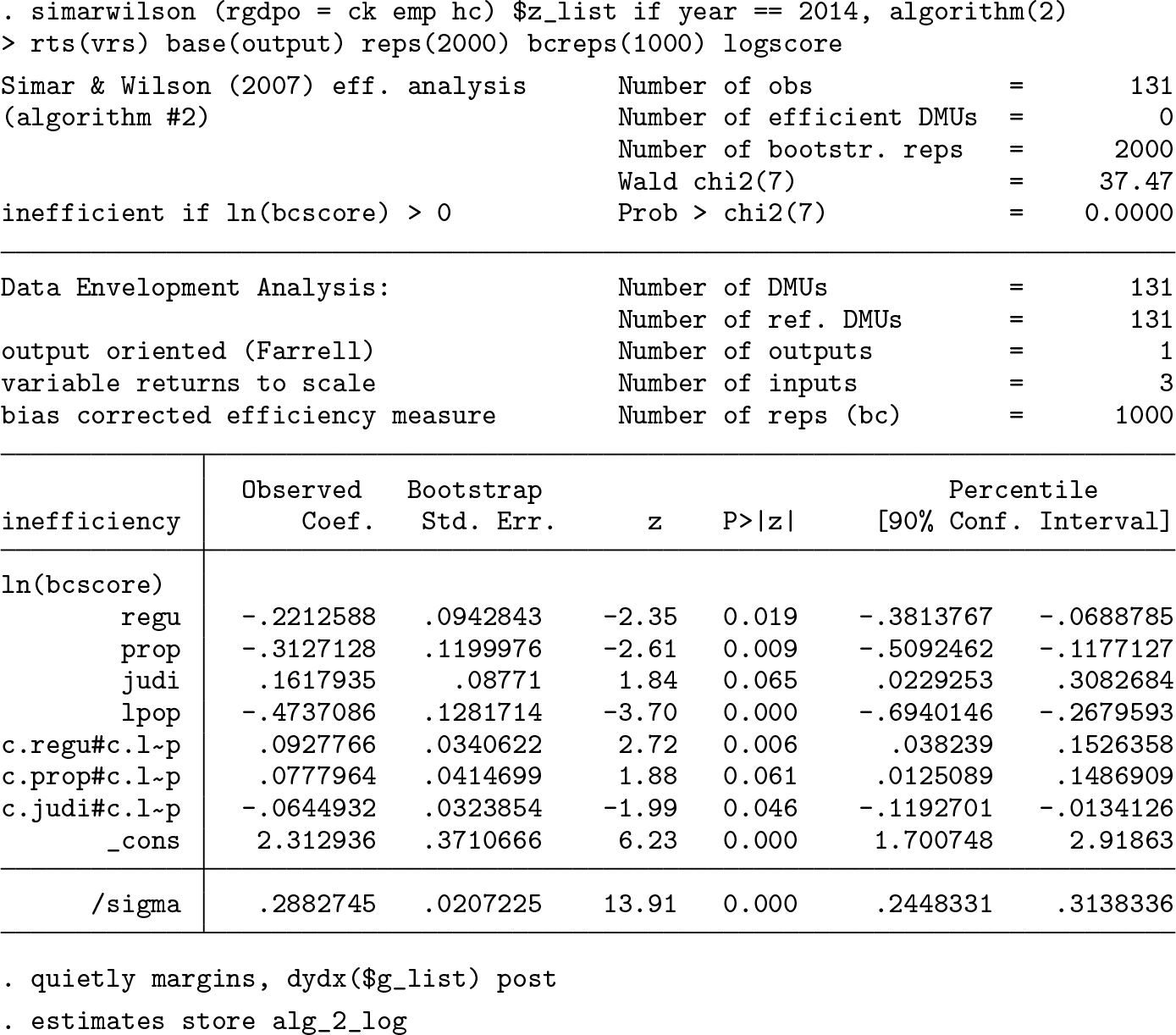
Then, we turn to algorithm(2). In this procedure, tailored, bias-corrected efficiency scores enter the regression model at the left-hand side. Hence, we cannot use externally estimated scores but instead let simarwilson carry out the bias correction internally. This requires the (rgdpo = ck emp hc) syntax and the options rts(vrs) and base(output). The last two determine the DEA model used. By specifying the option tebc(tebc_vrs_o), we save the estimated, bias-corrected efficiency scores for possible later use. We opt for 1,000 replications in the bias-correction bootstrap, which is well above the default suggested in Simar and Wilson (2007). Fitting this model takes 96 seconds. Because of the relatively small sample size, using algorithm(2) increases computing time by only 10%; compare footnote 16. Because we do not use externally estimated scores as the left-hand-side variable but let simarwilson run the DEA internally, the reported output also involves comprehensive information about the DEA model used.³¹ In this application, using bias-corrected instead of uncorrected scores has only a moderate impact on the estimated coefficients and the associated estimated confidence intervals.

summarize gives us descriptive statistics for estimated, bias-corrected inefficiency. Comparing them with the descriptives for te_vrs_o shows that the bias correction adjusts the estimated scores away from unity, ruling out (seemingly) fully efficient countries.

To interpret the results qualitatively, we examine the estimated mean marginal effects. This yields a rather clear picture. While, on average, the regulatory burden and judicial independence appear to be immaterial for the efficiency of GDP generation, the protection of property rights matters. Except for tobit, the estimated marginal effect is clearly significant and amounts to roughly 1/3 (Farrell, output-oriented) units, by which inefficiency is reduced in response to a one-unit increase in property rights protection. This appears to be a strong effect that corresponds to a shift from the median to the 27th percentile of the sample distribution of tebc_vrs_o.

Measuring effects in terms of Farrell (output-oriented) efficiency units appears not to be particularly telling. Hence, one may prefer a scaled efficiency measure that allows for interpreting marginal effects in terms of percentage points. Thus, one may switch to the Shephard efficiency measure. Switching from outputto input-oriented efficiency, which would also yield efficiency scores within the unit interval, does not have much appeal for this application. It would imply the thought experiment of reducing input consumption, which appears rather odd given that the national capital stock and human capital are among the input variables.

While switching to the Shephard measure was straightforward for algorithm(1)— one just has to use the reciprocal of te_vrs_o as the dependent variable—in this application, it causes difficulties with algorithm(2). As indicated by a warning issued by simarwilson (see below), the bias correction yields some negative scores; compare section 2.3. These are not used in the truncated regressions. Thus, only 127, not 131, countries enter the regression analysis. In qualitative terms, using the Shephard measure as the left-hand-side variable does not change the general pattern of results. As expected (see footnote 28), the signs of all coefficients are just reversed, and all coefficients remain statistically significant.

One may force simarwilson to use negative bias-corrected scores in the regression analysis by combining invert with the option notwosided. However, one accepts two inconsistencies by doing this. Besides allowing for negative efficiency scores, which arguably makes little sense, one makes simarwilson apply different truncation rules in different steps of the estimation procedure; see footnote 18. As can be seen from the output below, simarwilson points the user to this issue. Indeed, forcing simarwilson to consider the few observations with negative scores has a noticeable impact on the estimated coefficients.

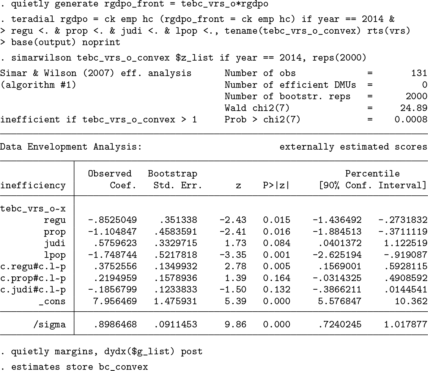
To specify a model that renders interpreting estimation results in quantitative terms more convenient, one can use the option logscore as a possible alternative to invert. By considering log inefficiency as the left-hand-side variable, one can interpret marginal effects as percentage reductions in inefficiency. Hence, we rerun our preferred model (algorithm 2, Farrell output-oriented efficiency) using the option logscore. The statistical significance and the signs of the estimated coefficients are equivalent to those from the specification of reference.

One may not feel comfortable with using a (bias-corrected) efficiency measure that conflicts with convexity of the production-possibility set; compare figure 1. One way of addressing this issue is to once again envelop the nonconvex bias-corrected estimated frontier with a convex hull and to use the distance to this convexified bias-corrected frontier as a dependent variable in the regression analysis (compare Badunenko, Henderson, and Russell [2013] and figure 5). The (ref_outputs = ref_inputs) specification of teradial allows one to straightforwardly implement this procedure; see the output below and Badunenko and Mozharovskyi (2016). Compared with its direct counterpart (simarwilson, algorithm(2) without invert and logscore), this once more adjusted efficiency measure changes the estimated coefficients markedly. Yet, qualitatively, the pattern of estimates remains the same.

Finally, we compare the marginal effects for all specifications of simarwilson that we have estimated. Somewhat surprisingly, unlike the specification of reference, the specifications using the Shephard measure argue for more regulatory interference for improving efficiency (p-values 0.039 and 0.096, respectively). One may hence speculate that regu captures both detrimental and beneficial facets of business regulation. In terms of the point estimates, all model specifications yield a positive association of property right protection and GDP efficiency. Only for the Shephard measure as the left-hand-side variable (without option notwosided) does the average marginal effect of prop turn statistically insignificant at the 10% level.

Using the Shephard measure (option invert) or the option logscore makes interpreting the estimated marginal effect easier. According to the specification using the Shephard measure (without notwosided), a one-unit increase in prop on average improves efficiency by 3.6 percentage points. According to the specification using log inefficiency at the left-hand side, the mean effect is a 10.7% reduction in inefficiency. With respect to judi, all estimated marginal effects are statistically insignificant. In terms of estimated average marginal effects, basing the analysis on a convex estimated hull has almost no effect compared with using the nonconvex, bias-corrected estimated frontier.

4.2 Effect heterogeneity

We complete our application by analyzing possible heterogeneity in the efficiency effects of burden of government regulation, property rights protection, and judicial independence. In doing this, we focus on simarwilson, algorithm(2) without invert and logscore as our preferred estimation method. The estimated mean marginal effects from this model suggest that only the protection of property rights matters for efficiency. However, this result might just be an artifact of averaging heterogeneous effects. We graphically examine possible effect heterogeneity using the marginsplot command; see [R] marginsplot and the output below. We consider two dimensions of heterogeneity: heterogeneity with respect to country size measured by lpop (figure 2, right panel) and heterogeneity with respect to the respective considered dimension of governance quality (figure 2, left panel).

Figure 2.

Estimated marginal effects of governance-quality indices on inefficiency by country size (right panel) and its respective own value (left panel). NOTE: Farrell output-oriented efficiency as dependent variable; Simar and Wilson (2007), algorithm 2 used for estimation; 90% confidence bands indicated by shaded areas. SOURCE: Calculations are our own, based on Penn World Table and World Economic Forum Global Competitiveness Report data.

The left panel of figure 2 does not suggest that the effect heterogeneity with respect to the respective category of governance quality is a big issue, at least qualitatively. The effects of both the burden of government regulation and judicial independence on inefficiency are statistically insignificant at any level of regu and judi. This is perfectly in line with the small and statistically insignificant estimated mean effects. Yet, if one focuses on the point estimates of the marginal effect of regu and for a moment ignores statistical significance, then figure 2 points to relaxing government regulation being beneficial if the regulator burden is high but exerting a negative effect on efficiency if it is already small. This pattern arguably makes sense. The pattern for property rights protection does also not conflict with what we found for the mean effect. Here we find a significant inefficiency-reducing effect of better property rights protection over the entire range of prop. Yet the effect seems to be much stronger for low levels of property rights protection, though the estimated marginal effect gets increasingly noisy for small values of prop.

The overall picture is somewhat different for heterogeneity with respect to country size (figure 2, right panel). There the marginal effect of all three governance indicators exhibits substantial heterogeneity. While focusing on mean marginal effects suggested that the level of regulation was immaterial for national efficiency, considering effect heterogeneity challenges this finding. More specifically, figure 2 suggests that relaxing government regulation reduces inefficiency in small countries. Yet in big countries, it seems to exert a negative effect on national efficiency. This pattern corroborates our earlier hypothesis of regulatory burden being an ambiguous concept because in certain circumstances some regulation may be well required for efficient production. A similar pattern of heterogeneity is found for the effect of prop. In small countries, improving the protection of property rights is clearly beneficial for efficiency of GDP production, while for big countries, such an effect is not found in the data. The reverse pattern of heterogeneity is found with respect to judicial independence. While the effect of judi on efficiency is statistically insignificant for many values of lpop, figure 2 suggests a statistically significant, efficiency-reducing effect for very small countries. However, this somewhat surprising finding has to be interpreted with caution. Near collinearity might be a technical explanation for the mirror-inverted patterns found for prop and judi. Both variables are strongly correlated (0.903) in the estimation sample, while their respective correlations with regu (0.506 and 0.448) are much weaker.

4.3 The gciget command

As mentioned in section 4.1, importing the indices from the Global Competitiveness Report that we used in our empirical study is not straightforward. We have developed the new command gciget to get the indices directly into the memory of Stata from the World Economic Forum’s Global Competitiveness Report.

gciget has three steps. First, it downloads the file GCI_Dataset_2007-2017.xlsx from the The Global Competitiveness Report section (http://reports.weforum.org/global-competitiveness-index-2017-2018/) of the World Economic Forum website. The user can optionally indicate the path to the Excel file GCI_Dataset_2007-2017.xlsx stored locally. Second, gciget imports the Excel file; see [D] import excel regarding the requirement for the version of Stata. Third, gciget processes the variables the user has specified after gciget. The resulting data are in a long format and are by default declared to be panel data; see [XT] xtset.

The syntax for gciget reads as follows:

gciget [varlist] [, clear noxtset noquery panelvar(newvar) url(filename) sheet("sheetname") cellrange([start]:[end]) nowarnings]

The user can optionally specify the varlist from the list of indices in the Global Competitiveness Report (see the Excel file GCI_Dataset_2007-2017.xlsx for the possible names). If no valid name of the index is specified, all indices will be processed.

The following options are available:

clear clears data in memory before loading the GCI data.

noxtset prevents loaded data from being declared panel data (see [XT] xtset). Without noxtset, gciget generates a new numeric panelvar, which is a numeric equivalent to the string variable countrycode. year serves as timevar.

noquery suppresses summary calculations by xtset. With noxtset, noquery has no effect.

panelvar(newvar) specifies the name of the numeric panelvar that is generated by gciget. The default is panelvar(cnNumber). With noxtset, panelvar() has no effect.

url(filename) specifies the URL of the GCI data. The default is url(http://www3.weforum.org/docs/GCR2017-2018/GCI_Dataset_2007-2017.xlsx). Specifying url(filename) might become necessary if a new version of the GCI is published and the name of the data file changes or if the web address changes for any other reason. url(filename) may also be used to specify the path to the GCI data, if the Excel file GCI_Dataset_2007-2017.xlsx has already been downloaded and locally stored.

sheet("sheetname") specifies the Excel worksheet to load. The default is sheet("Data"). Specifying sheet("sheetname") might become necessary if a new version of the GCI is published and the name of the relevant Excel worksheet changes. sheetname is passed through to import excel.

cellrange([start]:[end]) specifies a range of cells within the Excel sheet to load. The default is cellrange(A3:FM6527). Specifying cellrange( start :end ) might become necessary if a new version of the GCI is published and the structure of the Excel file changes. start:end is passed through to import excel.

nowarnings prevents gciget from displaying warnings that are routinely issued if the options url(filename), sheet("sheetname"), and cellrange( start :end ) deviate from the respective default.

gciget only helps the user get the data from the World Economic Forum into Stata. Thus, any liability for the data or their usage is disclaimed. That the data come from the World Economic Forum also puts restriction on the data availability and the terms and conditions under which the data can be used. As of this writing, the data are available for 2007–2017. The following code illustrates a simple import of four indices and plotting GCI for four countries.

. gciget EOSQ048 EOSQ051 GCI GCI.A.02.01, clear

Downloading the GCI_Dataset_2007-2017.xlsx file

Importing the GCI_Dataset_2007-2017.xlsx file

Processing EOSQ048: 1.09 Burden of government regulation, 1-7 (best) Processing EOSQ051: 1.01 Property rights, 1-7 (best)

Processing GCI: Global Competitiveness Index

Processing GCI_A_02_01: A. Transport infrastructure

. xtline GCI if countrycode == "USA" | countrycode == "DEU" |

> countrycode == "FRA" | countrycode == "GBR", overlay i(country)

> t(year) scheme(sj) xlabel(2007(2)2017)

. quietly graph export "GCI_four_cns.eps", as(eps) preview(off) replace

> fontface(Times)

Figure 3.

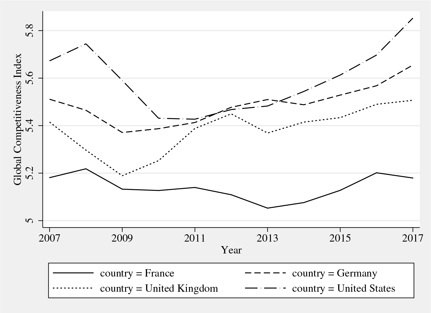
GCI for France, Germany, the UK, and the United States. Source: World Economic Forum’s Global Competitiveness Report.

5 Summary and conclusions

In this article, we introduced the new community-contributed command simarwilson, which implements Simar and Wilson (2007) two-stage efficiency analysis. This estimator has substantial value for applied efficiency analysis because it puts regression analysis of DEA scores on firm statistical ground. The new command extends the originally proposed procedure in some respects, which increases its applicability in applied empirical work. simarwilson complements the contributions of Ji and Lee (2010), Tauchmann (2012), and, particularly, Badunenko and Mozharovskyi (2016), who have already made related methods of nonparametric efficiency analysis available to Stata users.

8 Programs and supplemental materials

Supplemental Material, st0585 - Simar and Wilson two-stage efficiency analysis for Stata

Supplemental Material, st0585 for Simar and Wilson two-stage efficiency analysis for Stata by Oleg Badunenko and Harald Tauchmann in The Stata Journal

Footnotes

6 Acknowledgments

This work has been supported in part by the Collaborative Research Center “Statistical Modelling of Nonlinear Dynamic Processes” (SFB 823) of the German Research Foundation. The authors are grateful to Ramon Christen, Rita Maria Ribeiro Bastiao, Akash Issar, Ana Claudia Sant’Anna, Jarmila Curtiss, Meir José Behar Mayerstain, Erik Alda, Annika Herr, Hendrik Schmitz, Franziska Valder, Franz Josef Zorzi, Irina Simankova, Christian Merkl, Howard J. Newton, the participants of the 2015 German Stata Users Group meeting, and one anonymous reviewer for many valuable comments.

7 Supplementary figures

The figures below graphically illustrate the concepts of a restricted reference set (figure 4) and a convexified frontier () that were referred to in this article, using the same artificial data that were used to illustrate DEA in figure 1. Figure 4.

Estimated inefficiency for subsample of DMUs used as reference. Considering only a subsample of DMUs as reference set renders DMU B seemingly superefficient, both according to conventional $D E A ({\hat{θ}}_{B} = (y_{B}^{^{D E A *}} / y_{B}) < 1)$ and according to bias-corrected DEA $D E A ({\hat{θ}}_{B}^{b c} = (y_{B}^{^{b c *}} / y_{B}) < 1)$ . DMU A is still estimated to be inefficient; compare figure 1. Yet the magnitude of estimated inefficiency is somewhat smaller. NOTE: Artificial data generated in the same way as for figure 1. SOURCE: Calculations are our own.

Figure 5.

Convexified bias-corrected estimated frontier. Measuring inefficiency relative to the convexified bias-corrected frontier either does not affect estimated bias-corrected inefficiency (for example, DMU B) or increases estimated bias-corrected inefficiency (for example, DMU A). NOTE: Artificial data generated the same as figure 1. SOURCE: Calculations are our own.

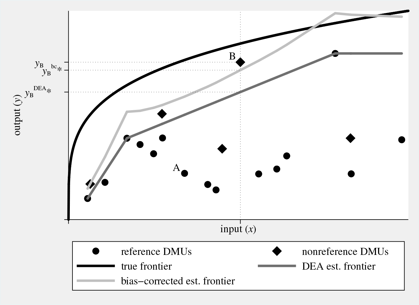
8 Programs and supplemental materials

To install a snapshot of the corresponding software files as they existed at the time of publication of this article, type

. net sj 19-4

. net install st0585 (to install program files, if available)

. net get st0585 (to install ancillary files, if available)

Notes

References

Aigner

D. J.

Lovell

C. A. K.

Schmidt

1977. Formulation and estimation of stochastic frontier production function models. Journal of Econometrics 6: 21–37.

Badunenko

Henderson

D. J.

Russell

R. R.

2013. Polarization of the worldwide distribution of productivity. Journal of Productivity Analysis 40: 153–171.

Badunenko

Mozharovskyi

2016. Nonparametric frontier analysis using Stata. Stata Journal 16: 550–589.

Banker

R. D.

Natarajan

2008. Evaluating contextual variables affecting productivity using data envelopment analysis. Operations Research 56: 48–58.

Charnes

Cooper

W. W.

Rhodes

1978. Measuring the efficiency of decision making units. European Journal of Operational Research 2: 429–444.

Chopin

2011. Fast simulation of truncated Gaussian distributions. Statistics and Computing 21: 275–288.

Chortareas

G. E.

Girardone

Ventouri

2013. Financial freedom and bank efficiency: Evidence from the European Union. Journal of Banking & Finance 37: 1223–1231.

Coelli

T. J.

Rao

D. S. P.

O’Donnell

C. J.

Battese

G. E.

2005. An Introduction to Efficiency and Productivity Analysis. 2nd ed. New York: Springer.

Cooper

W. W.

Seiford

L. M.

Tone

2007. Data Envelopment Analysis: A Comprehensive Text with Models, Applications, References and DEA-Solver Software. 2nd ed. New York: Springer.

10.

Daraio

Simar

2005. Introducing environmental variables in nonparametric frontier models: A probabilistic approach. Journal of Productivity Analysis 24: 93– 121.

11.

Daraio

2007. Advanced Robust and Nonparametric Methods in Efficiency Analysis: Methodology and Applications. New York: Springer.

12.

Emrouznejad

Yang

2018. A survey and analysis of the first 40 years of scholarly literature in DEA: 1978–2016. Socio-Economic Planning Sciences 61: 4–8.

13.

Farrell

M. J.

1957. The measurement of productive efficiency. Journal of the Royal Statistical Society, Series A 120: 253–290.

14.

Feenstra

R. C.

Inklaar

Timmer

M. P.

2015. The next generation of the Penn World Table. American Economic Review 105: 3150–3182.

15.

Fragkiadakis

Doumpos

Zopounidis

Germain

2016. Operational and economic efficiency analysis of public hospitals in Greece. Annals of Operations Research 247: 787–806.

16.

Glass

A. J.

Kenjegalieva

Taylor

2015. Game, set and match: Evaluating the efficiency of male professional tennis players. Journal of Productivity Analysis 43: 119–131.

17.

Hjalmarsson

Kumbhakar

S. C.

Heshmati

1996. DEA, DFA and SFA: A comparison. Journal of Productivity Analysis 7: 303–327.

18.

Hoff

2007. Second stage DEA: Comparison of approaches for modelling the DEA score. European Journal of Operational Research 181: 425–435.

19.

Y.-B.

Lee

2010. Data envelopment analysis. Stata Journal 10: 267–280.

20.

Kneip

Simar

Wilson

P. W.

2008. Asymptotics and consistent bootstraps for DEA estimators in nonparametric frontier models. Econometric Theory 24: 1663– 1697.

21.

Koopmans

T. C.

1951. An analysis of production as an efficient combination of activities. In Activity Analysis of Production and Allocation, ed. Koopmans

T. C.

, 33–97. New York: Wiley.

22.

McDonald

2009. Using least squares and tobit in second stage DEA efficiency analyses. European Journal of Operational Research 197: 792–798.

23.

Murillo-Zamorano

L. R.

2004. Economic efficiency and frontier techniques. Journal of Economic Surveys 18: 33–77.

24.

Pérez Urdiales

Lansink

A. O.

Wall

2016. Eco-efficiency among dairy farmers: The importance of socio-economic characteristics and farmer attitudes. Environmental & Resource Economics 64: 559–574.

25.

Ramalho

E. A.

Ramalho

J. J. S.

Henriques

P. D.

2010. Fractional regression models for second stage DEA efficiency analyses. Journal of Productivity Analysis 34: 239–255.

26.

Schwab

, ed. 2017. The Global Competitiveness Report 2017–2018. Geneva: World Economic Forum.

27.

Shephard

R. W.

1970. Theory of Cost and Production Functions. Princeton, NJ: Princeton University Press.

28.

Simar

Wilson

P. W.

2000. A general methodology for bootstrapping in nonparametric frontier models. Journal of Applied Statistics 27: 779–802.

29.

Simar

2007. Estimation and inference in two-stage, semi-parametric models of production processes. Journal of Econometrics 136: 31–64.

30.

Simar

2011. Two-stage DEA: Caveat emptor. Journal of Productivity Analysis 36: 205–218.

31.

Tauchmann

2012. Partial frontier efficiency analysis. Stata Journal 12: 461–478. World Economic Forum. 2018. The global competitiveness index dataset 2007–2018. http://www3.weforum.org/docs/GCR2017-2018/GCI_Dataset_2007-2017.xlsx.

Supplementary Material

Please find the following supplemental material available below.

For Open Access articles published under a Creative Commons License, all supplemental material carries the same license as the article it is associated with.

For non-Open Access articles published, all supplemental material carries a non-exclusive license, and permission requests for re-use of supplemental material or any part of supplemental material shall be sent directly to the copyright owner as specified in the copyright notice associated with the article.

0.00 MB