Multilevel mixed-effects parametric survival analysis: Estimation,simulation,and application

Abstract

In this article, I present the community-contributed stmixed command for fitting multilevel survival models. It serves as both an alternative to Stata’s official mestreg command and a complimentary command with substantial extensions. stmixed can fit multilevel survival models with any number of levels and random effects at each level, including flexible spline-based approaches (such as Royston–Parmar and the log-hazard equivalent) and user-defined hazard models. Simple or complex time-dependent effects can be included, as can expected mortality for a relative survival model. Left-truncation (delayed entry) is supported, and t-distributed random effects are provided as an alternative to Gaussian random effects. I illustrate the methods with a commonly used dataset of patients with kidney disease suffering recurrent infections and a simulated example illustrating a simple approach to simulating clustered survival data using survsim (Crowther and Lambert 2012, Stata Journal 12: 674–687; 2013, Statistics in Medicine 32: 4118–4134). stmixed is part of the merlin family (Crowther 2017, arXiv Working Paper No. arXiv:1710.02223; 2018, arXiv Working Paper No. arXiv:1806.01615).

1 Introduction

Clustered survival data are often observed in many settings. Within medical research, a common example is the analysis of recurrent-event data, where individual patients can experience the event of interest multiple times throughout the follow-up period, and the inherent correlation within patients can be accounted for using a frailty term (Gutierrez 2002).

In the field of meta-analysis, applications of individual patient data meta-analysis to survival data are growing because it is recognized as the gold standard approach (Simmonds et al. 2005). Analyzing the individual patient data simultaneously within a hierarchical structure allows direct adjustment for confounders and incorporation of nonproportional hazards in covariate effects (Smith, Williamson, and Marson 2005; Crowther et al. 2012; Crowther, Look, and Riley 2014). Often, a random treatment effect is assumed to account for heterogeneity present in treatment effects across the pooled trials.

A further area of interest is relative survival. Particularly prevalent in cancer survival studies, relative survival allows the modeling of excess mortality associated with a diseased population compared with that of the general population (Dickman et al. 2004). Such data often exhibit a hierarchical structure with patients nested within geographical regions such as counties. Patients living in the same area may share unobserved characteristics, such as environmental aspects or medical care access (Charvat et al. 2016).

With the release of Stata 14 came the mestreg command to fit multilevel mixedeffects parametric survival models, assuming normally distributed random effects and fit with maximum likelihood using Gaussian quadrature. In this article, I present the community-contributed stmixed command for fitting multilevel survival models. stmixed serves as both an alternative to mestreg and a complimentary command with substantial extensions. It can fit multilevel survival models with any number of levels and random effects at each level, including flexible spline-based approaches (such as Royston–Parmar and the log-hazard equivalent) and user-defined hazard models. Simple or complex time-dependent effects can be included, as can expected mortality for a relative survival model. Left-truncation (delayed entry) can be used, and t-distributed random effects are provided as an alternative to Gaussian random effects. stmixed can fit a multilevel survival model with any of the aforementioned extensions and can be combined with a user-defined hazard model to provide a platform for methods development within a survival context.

In essence, stmixed is now a wrapper command for the recently introduced merlin command (Crowther 2017, 2018), which provides a general framework for fitting multivariate mixed-effects models. Multilevel survival models are one of the many classes of models that merlin can fit; however, to make the methods more accessible to researchers, I provide stmixed as a convenient wrapper command with a far simpler syntax yet still with the power and flexibility of merlin.

This article is arranged as follows. Section 2 describes the multilevel parametric survival framework and derives the likelihood used to fit the models, including the extension to relative survival models as well as left-truncation (delayed entry). Section 3 details the model syntax of stmixed and describes the available options. Section 4 describes the postestimation tools available. Section 5 illustrates the command with a dataset of patients with kidney disease who are followed up with for recurrent infection at the catheter-insertion point; this section also shows how to simulate clustered survival data using the survsim command, representing an individual patient data meta-analysis scenario with a random treatment effect. Section 6 concludes the article.

2 Multilevel mixed-effects survival models

For ease of exposition, I describe the methods in the context of a two-level model, but stmixed can handle any number of levels. I begin with some notation. Define $i=1, . . . , N$ clusters (for example, trials or centers) with each cluster having $j=1, . . . , n_i$ patients. Let S_ij be the true survival time of the jth patient in the ith cluster, let $T_{ij}=min(S_{ij}, C_{ij})$ be the observed survival time, and let C _ij be the censoring time. I define an event indicator, d _ij, which takes the value of 1 if $S_{ij}\le C_{ij}$ and 0 otherwise.

2.1 Proportional-hazards parametric survival models

The proportional-hazards mixed-effects survival model can be written as

$h_{ij}(t) =h_0(t) exp\hspace{0.17em}(x_{ij}^T\beta +z_{ij}^T{b}_j)$

1

where h ₀(t) is the baseline hazard function of a standard parametric model, such as the exponential, Weibull, or Gompertz distribution; a more general spline-based approach, such as using restricted cubic splines on the log-hazard scale (Bower, Crowther, and Lambert 2016); or even a user-defined function. I define design matrices x _ij and z _ij for the fixed (β) and random (b _j) effects, respectively. I assume the random effects follow a multivariate normal distribution with $b_j~N(0,\Sigma )$ (stmixed also allows multivariate t-distributed random effects). If $z_{ij}=1$ for all i and j, then (1) reduces to a shared frailty model, such as those available in streg, albeit with a different choice of frailty distribution.

2.2 Flexible parametric models

An alternative to the standard proportional-hazards distribution is the flexible parametric model of Royston and Parmar (2002) modeled on the cumulative hazard scale, which has recently been extended to incorporate random effects by Crowther, Look, and Riley (2014). Therefore,

$H_{ij}(t) =H_0(t) exp\hspace{0.17em}(x_{ij}^T\beta +z_{ij}^T{b}_j)$

where H ₀(t) is the cumulative baseline hazard function. The spline basis for this specification is derived from the log cumulative-hazard function of a Weibull proportional hazards model. The linear relationship with log time is relaxed through the use of restricted cubic splines. Further details can be found in Royston and Parmar (2002) and Royston and Lambert (2011). On the log cumulative-hazard scale, we have

$log\{H_{ij}(t)\}={\eta }_{ij}(t) =s\{log(t)|\gamma ,k_0\}+x_{ij}^T\beta +z_{ij}^T{b}_j$

2

where s(·) are our basis functions with knot vector k ₀. Transforming to the hazard and survival scales gives

$h_{ij}(t) =\left[\frac{1}{t}\hspace{0.17em}\frac{ds\{log(t)|\gamma ,k_0\}}{dlog(t)}\right] exp\{{\eta }_{ij}(t)\}, S_{ij}(t) =exp [-exp\{{\eta }_{ij}(t)\}]$

In this framework, I am assuming proportional cumulative hazards. However, this in fact implies proportional hazards as in the models described in section 2.1.

Nonproportional (cumulative) hazards

Relaxing the assumption of proportional hazards allows the investigation of whether the effect of a covariate changes with time. This is called nonproportional hazards or time-dependent effects, the occurrence of which is commonplace in the analysis of survival data. Examples include treatment effects that vary over time (Mok et al. 2009); in registry-based studies, where follow-up can be substantial, covariate effects have been found to vary (Lambert et al. 2011).

Nonproportional cumulative hazards have been incorporated into the flexible parametric framework by Royston and Parmar (2002), achieved by interacting covariates with spline functions of log time and including them in the linear predictor (Lambert and Royston 2009). This provides even greater flexibility in capturing complex effects that are not restricted to linear functions of time. Equation (2) becomes

$log\{H_{ij}(t)\}={\eta }_{ij}(t) =s\{log(t)|\gamma ,k_0\}+x_{ij}^T\beta +z_{ij}^T{b}_j+{\displaystyle \sum _{r=1}^{R}s\{log(t)|{\delta }_r,k_r\}{x}_{ijr}}$

Each time-dependent effect can have a varying number of spline terms, depending on the number of knots, k _r.

Within stmixed, time-dependent effects using restricted cubic splines can be used with all available models.

2.3 User-defined survival models

stmixed also allows the user to provide their own definitions for the hazard function, with or without also defining a cumulative hazard function, to allow the use of bespoke survival models with general hazard functions. For estimation, both the hazard and the cumulative hazard functions are required (see section 2.5 for further details), so when only the hazard is provided, the cumulative hazard function is calculated using numerical integration. Such a general implementation allows the user complete flexibility while still allowing him or her to use the random-effects engine within stmixed, which also syncs with the relative survival extension and delayed entry. More details on writing a user-defined function can be found in Crowther (2018).

2.4 Relative survival

Relative survival allows us to model the excess mortality associated with a diseased population compared with that of the general population, matched appropriately on the main factors associated with patient survival, such as age and gender (Dickman et al. 2004). For a recent extensive description and implementation of the tools available for relative survival analysis in Stata, along with a description of the differing approaches, see Dickman and Coviello (2015) and references therein.

Concentrating on applications of relative survival to cancer settings, the data generally come from population-based registries. Such data often exhibit a hierarchical structure with patients nested within geographical regions such as counties. Patients living in the same area may share unobserved characteristics, such as environmental aspects or medical care access. Charvat et al. (2016) recently described a flexible relative survival model allowing a random intercept, with the baseline log-hazard function modeled with B-splines or restricted cubic splines. In this article, I extend the multilevel Royston–Parmar survival model described in Crowther, Look, and Riley (2014) and essentially any other hazard-based survival model to the relative survival setting, further allowing any number of random effects, including random coefficients. Modeling on the log cumulative-hazard scale avoids the need for numerical integration, which is required when modeling on the log-hazard scale with splines and will generally require fewer spline terms than when modeling on the log-hazard scale.

Within a multilevel modeling framework, I therefore define the total hazard at the time since diagnosis, t, for the jth patient in the ith cluster (area) to be h _ij(t), with

$h_{ij}(t) =h_{ij}^{*}(t) +{\lambda }_{ij}(t)$

where

$h_{ij}^{*}(t)$ is the expected mortality for the jth patient in the ith cluster,

${\lambda }_{ij}(t)$ is the excess mortality for the jth patient in the ith cluster,

and our model is

${\lambda }_{ij}(t) ={\lambda }_0(t) exp(X_{ij}^T\beta +Z_{ij}^T{b}_i)$

where λ ₀(t) is the baseline hazard function with available choices including exponential, Weibull, Gompertz, spline based, or user defined.

Alternatively, I could model on the (log) cumulative excess-hazard scale using the flexible parametric model of Royston and Parmar (2002), where I define the total cumulative hazard at the time since diagnosis, t, for the jth patient in the ith cluster (area) to be H _ij(t), with

$H_{ij}(t) =H_{ij}^{*}(t) + {\Lambda }_{ij}(t)$

where

$H_{ij}^{*}(t)$ is the expected cumulative mortality for the jth patient in the ith cluster,

${\Lambda }_{ij}(t)$ is the excess cumulative mortality for the jth patient in the ith cluster,

and our model is

${\Lambda }_{ij}(t) ={\Lambda }_0(t) exp(X_{ij}^T\beta +Z_{ij}^T{b}_i)$

where Λ₀(t) is the baseline cumulative hazard function modeled with restricted cubic splines.

2.5 Likelihood and estimation

Defining the likelihood for the ith cluster under the mixed-effects framework, we have

$L_i(\theta ) ={\displaystyle {\int }_{-\infty }^{\infty }\left\{{\displaystyle \prod _{j=1}^{n_i}p(T_{ij}, d_{ij}|b_i,\theta )}\right\}}\hspace{0.17em}p(b_i|\theta ) d{b}_i$

3

with parameter vector θ. Under a hazard-scale model,

$p(T_{ij}, d_{ij}|b_i,\theta )=h{(T_{ij})}^{d_{ij}} exp\left\{-{\displaystyle {\int }_0^{T_{ij}}h(u) du}\right\}$

4

with h(T _ij) defined in (1). Under the flexible parametric survival model,

$p(T_{ij}, {\text{d}}_{ij}|b_i,\theta )={\left(\left[\frac{1}{T_{ij}}\hspace{0.17em}\frac{ds\{\text{log}(T_{ij})|\gamma ,k_0\}}{d log(T_{ij})}\right]exp({\eta }_{ij})\right)}^{d_{ij}} exp\{-exp({\eta }_{ij})\}$

5

Finally, I assume the random effects follow a multivariate normal distribution

$p(b_i|\theta ) ={(2\pi |\Sigma |)}^{-q/2}exp\left(\frac{-{b^{\prime }}_j\hspace{0.17em}{\Sigma }^{-1}{b}_j}{2}\right)$

with variance–covariance matrix Σ and number of random effects q. The (possibly multidimensional) integral in (3) is analytically intractable, requiring numerical techniques to evaluate. stmixed uses either m-point mean-variance adaptive or nonadaptive Gauss– Hermite quadrature (Pinheiro and Bates 1995; Rabe-Hesketh, Skrondal, and Pickles 2002; Liu and Huang 2008) or Monte Carlo integration. The default estimation method first fits the appropriate fixed-effects model followed by the full model with variance and covariance parameters given starting values of 0 and 1, respectively. stmixed also allows multivariate t-distributed random effects with specified degrees of freedom, in which case only Monte Carlo integration is supported.

2.6 Relative survival likelihood

The adaptation to the likelihood in (3) to turn it into a relative survival model is relatively simple. All that is needed is the expected mortality rate at each event time, which is usually obtained from national or regional life tables. Under a hazard-scale model, (4) becomes

$p(T_{ij}, d_{ij}|b_i,\theta )=\hspace{0.17em}{\{h^{*}(T_{ij}) +\hspace{0.17em}\hspace{0.17em}\lambda (T_{ij})\}}^{d_{{ }^{ij}}}exp\left\{-{\displaystyle {\int }_0^{T_{ij}}\lambda (u) du}\right\}$

and under a cumulative hazard-scale model, (5) becomes

$p(T_{ij}, d_{ij}|b_i,\theta )=\hspace{0.17em}{\left[h^{*}(T_{ij})\hspace{0.17em}\hspace{0.17em}+\hspace{0.17em}\hspace{0.17em}\left\{\frac{1}{T_{ij}}\hspace{0.17em}\hspace{0.17em}\frac{ds\{log(T_{ij})|\gamma ,k_0\}}{d log(T_{ij})}\right\}exp({\eta }_{ij}) \right]}^{d_{ij}}exp\{-exp({\eta }_{ij})\}$

which provides substantial extensions to the relative survival literature.

2.7 Left-truncation and delayed entry

The addition of left-truncation and delayed entry within a random-effects survival setting raises a particular extra level of complexity. The random-effects distributions are defined at t = 0. As such, the left-truncation time point is conditional on each patient’s subject-specific random-effects contributions. For more details, I refer the reader to van den Berg and Drepper (2016). Our likelihood function becomes

$L_i(\theta |T_{0i}) =\frac{{\displaystyle {\int }_{-\infty }^{{ }_{\infty }}\left\{{\displaystyle \prod _{j=1}^{n_i}p(T_{ij}, d_{ij}|b_i,\theta )}\right\}p(b_i|\theta ) d{b}_i}}{S(T_{0i}|\theta )}$

6

where S(T _{0 i}|θ) is the marginal survival function at the entry time T _{0 i}, defined as

$S(T_{0i}|\theta ) ={\displaystyle {\int }_{-\infty }^{\infty }S(T_{0i}|b_i,\theta )p(b_i|\theta ) d{b}_i}$

Thus, there are two sets of analytically intractable integrals to evaluate in (6), which increases computation time.

3 The stmixed command

3.1 Syntax

stmixed [varlist] [if] [in] || re_equation [|| re_equation…] [, noconstant distribution(string) df(#) knots(numlist) tvc(varlist) dftvc(numlist) knotstvc(numlist) bhazard(varname) covariance(vartype) intmethod(intmethod) intpoints(#) adaptopts(adaptopts) from(matname) restartvalues(sv_list) apstartvalues(#) zeros maximize_options showmerlin level(#) ]

and the syntax of re_equation is

levelvar: [varlist] [, noconstant]

stmixed requires that your data are stset.

3.2 Options

Model

noconstant suppresses the constant (intercept) term and may be specified for the fixedeffects equation and random-effects equations.

distribution(string) specifies the survival distribution.

distribution(exponential) fits an exponential survival model.

distribution(weibull) fits a Weibull survival model.

distribution(gompertz) fits a Gompertz survival model.

distribution(rp) fits a Royston–Parmar survival model. This is a highly flexible, fully parametric alternative to the Cox model, modeled on the log cumulativehazard scale using restricted cubic splines.

distribution(rcs) fits a log-hazard scale flexible parametric survival model. This is a highly flexible, fully parametric alternative to the Cox model, modeled on the log-hazard scale using restricted cubic splines.

distribution(user, user_functions) specifies a user-defined survival model; see help merlin user-defined functions.

df(#) specifies the degrees of freedom for the restricted cubic spline function used for the baseline function under an rp or rcs survival model. # must be between 1 and 10, but a value between 1 and 5 is usually sufficient. The knots() option is not applicable if df() is specified. The knots are placed at the evenly spaced centiles of the distribution of the uncensored log survival-times. These are interior knots, and there are also boundary knots placed at the minimum and maximum of the distribution of uncensored survival times.

knots(numlist) specifies knot locations for the baseline distribution function under an rp or rcs survival model as opposed to the default locations set by df(). The locations of the knots are on the standard time scale. However, the scale used by the restricted cubic spline function is always log time. Default knot positions are determined by the df() option.

tvc(varlist) gives the name of the variables that have time-varying coefficients. Time-dependent effects are fit using restricted cubic splines. The degrees of freedom is specified using the dftvc() option.

dftvc(numlist) gives the degrees of freedom for each time-dependent effect in tvc(), in matching order.

knotstvc(numlist) defines numlist as the location of the interior knots for time-dependent effects.

bhazard(varname) specifies the variable that contains the expected mortality rate, which invokes a relative survival model.

covariance(vartype) specifies the structure of the covariance matrix for the random effects. vartype may be diagonal, exchangeable, identity, or unstructured. The default is covariance(diagonal).

covariance(diagonal) allows a distinct variance for each random effect within a random-effects equation and assumes that all covariances are 0.

covariance(exchangeable) allows common variances and one common pairwise covariance.

covariance(identity) is short for “multiple of the identity”; that is, all variances are equal and all covariances are 0.

covariance(unstructured) allows for all variances and covariances to be distinct. If an equation consists of p random-effects terms, the unstructured covariance matrix will have p(p + 1)/2 unique parameters.

Integration

intmethod(intmethod), intpoints(#), and adaptopts(adaptopts) affect how integration for the latent variables is numerically calculated.

intmethod(intmethod) specifies the method and defaults to intmethod(mvaghermite). The current implementation uses mean-variance adaptive quadrature at the highest level and nonadaptive quadrature at lower levels. Sometimes, it is useful to fall back on the less computationally intensive and less accurate intmethod(ghermite) and then perhaps use one of the other more accurate methods. intmethod(mcarlo) tells stmixed to use Monte Carlo integration, which uses either Halton sequences with normally distributed random effects or antithetic random draws with t-distributed random effects.

intpoints(#) specifies the number of integration points to use. This option defaults to intpoints(7) with intmethod(ghermite) and intmethod(mvaghermite); it defaults to intpoints(150) with intmethod(mcarlo). Increasing the number increases accuracy but also increases computational time. Computational time is roughly proportional to the number specified.

adaptopts(adaptopts) affects the adaptive part of adaptive quadrature (another term for numerical integration) and thus is relevant only for intmethod(mvaghermite). The default is adaptopts(nolog iterate(1001)). adaptopts are the following:

[no] log specifies whether iteration logs are shown each time a numerical integral is calculated.

iterate(#) specifies the number of iterations to update the integration points, which will include updating prior to iteration 0 in the maximization process.

Estimation

from(matname) allows you to specify starting values.

restartvalues(sv_list) allows you to specify starting values for specific random-effects variances. See help merlin estimation for further details.

apstartvalues(#) allows you to specify a starting value for all ancillary parameters, that is, those defined using the nap() option. See help merlin estimation for further details about the nap() option.

zeros tells stmixed to use 0 for all parameters’ starting values rather than fit the fixedeffects model. Both restartvalues() and apstartvalues() may be used with zeros.

maximize options: difficult, technique(algorithm spec), iterate(#), [no]log, trace, gradient, showstep, hessian, shownrtolerance, tolerance(#), ltolerance(#), gtolerance(#), nrtolerance(#), nonrtolerance, from(init specs); see [R] Maximize. These options are seldom used, but the difficult option may be useful if there are convergence problems.

Reporting

showmerlin displays the merlin syntax used to fit the model.

level(#) specifies the confidence level, as a percentage, for confidence intervals (CIs). The default is level(95) or as set by set level.

4 stmixed postestimation

4.1 Syntax for obtaining predictions

predict newvar [if] [in] [, eta hazard survival chazard cif rmst timelost fixedonly marginal at(varname # [varname # …]) ci timevar(varname) level(#)]

4.2 Options

Note that if a relative survival model has been fit using the bhazard() option, then “survival” refers to relative survival and “hazard” refers to excess hazard.

eta calculates the expected value of the linear predictor.

hazard calculates the predicted hazard.

survival calculates each observation’s predicted survival probability.

chazard calculates the predicted cumulative hazard.

cif calculates the predicted cumulative incidence function.

rmst calculates the restricted mean survival time, that is, the integral of the survival function up to time t.

timelost calculates the time lost due to the event occurring, that is, the integral of the cumulative incidence function up to time t.

fixedonly specifies predictions based on the fixed portion of the model.

marginal specifies predictions calculated marginally with respect to the random effects, that is, population-averaged predictions.

at(varname # varname # … ) requests that the covariates specified by the listed variable name or names be set to the listed # values. For example, at(x1 1 x3 50) would evaluate predictions at x1 = 1 and x3 = 50. This is a useful way to obtain out-of-sample predictions.

ci calculates the CI for the requested statistic and stores the lower and upper limits in newvar_lci and newvar_uci, respectively. The delta method is used in all calculations using predictnl.

timevar(varname) defines the variable used as time in the predictions. This is useful, for example, for large datasets where, for plotting purposes, predictions are needed only for 200 observations. Use this option with care because predictions may be made at whatever covariate values are in the first 200 rows of data. This can be avoided by using the at() option to define the covariate patterns for which you require the predictions. The default is timevar(_t).

level(#) specifies the confidence level, as a percentage, for CIs. The default is level(95) or as set by set level.

5 Examples

In this section, I illustrate the command in two areas of research, namely, recurrent-events analysis and the individual participant data meta-analysis of survival data.

5.1 Recurrent event data

I consider the commonly used catheter.dta, consisting of 38 patients with kidney disease (McGilchrist and Aisbett 1991). The outcome of interest is infection at the catheter-insertion point, with our baseline being time of initial catheter insertion. Patients experience up to two recurrences of infection, resulting in a total of 58 events. In the examples, I use the Royston–Parmar model for illustration. I initially fit a null model—that is, no covariates and no random effects—to select the degrees of freedom for the baseline cumulative-hazard function, using the Akaike information criterion to guide the choice. This selected 3 degrees of freedom (not shown), clearly indicating the need for a flexible spline-based model to capture the complex hazard function.

I now fit a Royston–Parmar proportional hazards model with a normally distributed frailty, adjusting for age and gender:

Random effects are named with an M and a number. Therefore, stmixed first provides some text ensuring the user can understand which random effects correspond to what. It also reports creating some spline variables named rcs1_#, which are the baseline splines for the Royston–Parmar model. The estimation procedure by default fits the fixed-effects-only model to obtain starting values for the full model. Random-effects variances are given a starting value of 1 with any covariances given a starting value of 0.

The model estimates a hazard ratio of 0.231 (95% CI: [0.088, 0.606]) for a female compared with a male of the same age and a nonstatistically significant age effect (note coefficients in the results table are log hazard-ratios). The estimated frailty standard deviation is 0.801 (95% CI: [0.411, 1.563]), indicating a highly heterogeneous baseline hazard function.

We can relax the assumption of proportional hazards by forming an interaction between a covariate of interest and a function of time. stmixed allows an interaction between covariates and a restricted cubic spline function of log time through the tvc(), dftvc(), and knotstvc() options. For example, we form an interaction between log time (dftvc(1)) and female:

Given the statistically significant interaction, we observe evidence of nonproportionality in the effect of female. There is substantial flexibility in being able to model nonproportional hazards in any number of covariates with differing degrees of freedom.

Predictions

A variety of predictions can be obtained following the fitting of a model. I can obtain the predicted survival function, shown in figure 1 with 95% CI, based on the fixed portion of the model for a 45-year-old female through use of the at() option, as follows:

. predict s1, survival ci at(age 45 female 1)

note: confidence intervals calculated using Z critical values

which can be plotted by

Figure 1.

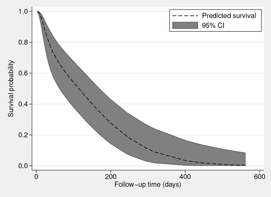
Predicted survival for a 45-year-old female based on the fixed portion of the model

To compare across covariate patterns—for example, to assess the impact of gender— we can predict restricted mean survival by typing

. predict rmst_male, rmst marginal ci at(age 45 female 0) note: confidence intervals calculated using Z critical values

. predict rmst_female, rmst marginal ci at(age 45 female 1) note: confidence intervals calculated using Z critical values

and plotting

. twoway (rarea rmst_male_lci rmst_male_uci _t, sort)

> (line rmst_male _t, sort)

> (rarea rmst_female_lci rmst_female_uci _t, sort)

> (line rmst_female _t, sort)

> , ylabel(,angle(h) format(%2.1f))

> xtitle("Follow-up time (days)")

> ytitle("Restricted mean survival time")

> legend(order(2 "Male" 4 "Female"))

Figure 2.

Restricted mean survival for a male or female aged 45

Figure 2 shows restricted mean survival as a function of time for a male or female patient with the same age of 45. The impact of being female is shown clearly, indicating that females live substantially longer than males of the same age.

5.2 Individual participant data meta-analysis of survival data

In this example, I will illustrate a simple approach to simulating clustered survival data, in the setting of an individual patient data meta-analysis of survival data through use of the survsim command (Crowther and Lambert 2012, 2013). I assume a scenario where I have data from 30 trials, each with 100 patients. Each trial compared a treatment with a control, with a 50% probability of being assigned to each arm. I assume that the treatment effect for each trial comes from a normal distribution, N(−0.5, 0.5²)—that is, an average log hazard-ratio of −0.5 (hazard ratio = exp(−0.5) = 0.607)—with a heterogeneity standard deviation of 0.5. I assume a Weibull baseline hazard function, with scale and shape parameter values of λ = 0.1 and γ = 1.2, indicating 50.2% survival in the control group after five years, at which time administrative censoring is assumed.

A key trick to note here is that in the survsim command, I included the variable trteffectsim and assigned it a coefficient value of 1. This allows for seamless incorporation of random effects on covariates that are included in the linear predictor and multiplied by a coefficient of 1. Then, when the model is fit using stmixed, the trt variable is used, which indicates treatment group.

In the stmixed model fit, I enter trt as both a fixed and a random effect, but I use the noconstant option to indicate no random intercept. This is a rather restrictive model because it assumes that each trial has the same baseline hazard function. In practice, you may include the trialid variable in the linear predictor to allow proportional trial effects, stratify by trial membership to allow separate trial effects (Crowther et al. 2012; Crowther, Look, and Riley 2014), or allow a random intercept at the trial level.

6 Conclusion

In this article, I introduced the stmixed command for multilevel mixed-effects survival analysis. stmixed provides substantial extensions to mestreg, including flexible spline-based survival models, user-defined survival models, the extension to relative multilevel survival, simple or complex time-dependent effects, and t-distributed random effects. I hope the many survival models available will be useful in applied research.

Given that stmixed is essentially a shell file for merlin, any improvements that are implemented in merlin will filter up to stmixed.

7 Programs and supplemental materials

Supplemental Material, st0584 - Multilevel mixed-effects parametric survival analysis: Estimation, simulation, and application

Supplemental Material, st0584 for Multilevel mixed-effects parametric survival analysis: Estimation, simulation, and application by Michael J. Crowther in The Stata Journal