Performance simulations for categorical mediation: Analyzing khb estimates of mediation in ordinal regression models

Abstract

Standard mediation techniques for fitting mediation models cannot readily be translated to nonlinear regression models because of scaling issues. Methods to assess mediation in regression models with categorical and limited response variables have expanded in recent years, and these techniques vary in their approach and versatility. The recently developed khb technique purports to solve the scaling problem and produce valid estimates across a range of nonlinear regression models. Prior studies demonstrate that khb performs well in binary logistic regression models, but performance in other models has yet to be investigated. In this article, we evaluate khb‘s performance in fitting ordinal logistic regression models as an exemplar of the wider set of models to which it applies. We examined performance across 38,400 experimental conditions involving sample size, number of response categories, distribution of variables, and amount of mediation. Results indicate that under all experimental conditions, khb estimates the difference (mediation) coefficient and its associated standard error with little bias and that the nominal confidence interval coverage closely matches the actual. Our results suggest that researchers using khb can assume that the routine reasonably approximates population parameters.

1 Introduction

Researchers are often interested in conducting mediation analysis for categorical response variables (for convenience, we speak of “mediation” throughout, although this process is generally statistically indistinguishable from spuriousness). Because categorical response variables present a more complex problem than in linear regression models, several solutions have been proposed to resolve the longstanding issues of scaling (Erikson et al. 2005; Buis 2010). A relatively new approach commonly known as khb has grown rapidly in popularity since introduction by Kohler, Karlson, and Holm (2011). Despite wide use in various disciplines—with some 1,400 citations to the foundational khb articles by September 2019 (Kohler, Karlson, and Holm 2011; Karlson and Holm 2011; Breen, Karlson, and Holm 2013, Forthcoming, 2018; Karlson, Holm, and Breen 2012—the previous performance evaluations of khb were restricted to binary response models (Karlson and Holm 2011; Karlson, Holm, and Breen 2012; Best and Wolf 2012) and encompassed a relatively modest set of conditions (sample size, degree of mediation).

While the current Stata implementation of the khb approach can be applied to over 13 different procedures besides the binary response model (ordinal logit, multinomial logit, rank ordered logit, xtlogit, etc.), we cannot analyze all of these models; rather, we focus on the ordinal logit model. Using bootstrapping simulations, we simulated a range of data conditions and evaluated the performance of the khb package across these experimental conditions. In this analysis, we make several important contributions.

First, no evaluation of the performance of the khb approach applied to ordinal response models exists in previous literature. In fact, despite regression models for ordinal response variables being widespread in the sociobehavioral and biomedical sciences, performance analyses of such models even in simple applications (that is, without mediation estimates) are essentially absent from the literature except for the work of Lipsitz et al. (2013) on bias correction for parameter estimates in ordered logistic regression. With such paucity of literature on ordinal response-model performance, the existing evidence is insufficient to conclude that previous work about the performance of khb with binary variables necessarily applies to ordinal responses.

Second, estimation performance with an ordinal rather than binary response variable arguably presents a more difficult test for the khb method, although no one has yet empirically or theoretically examined this question. Our suspicion here rests first on noting that a k-category ordinal response variable always requires estimation of $k-\text{2}$ more threshold parameters than the corresponding binary model. Further, for the least sparse situation of a uniformly distributed response variable, an ordinal model with given N will have 2/k proportionally fewer observations (“events”) to fill each category than its binary response peer. Concerns about sparsity should be even worse in actual research practice because ordinal response data so commonly show skewed or other nonuniform distributions with substantially fewer observations in one or more extreme categories than in others. This potential for sparsity has been a common emphasis in evaluations of the effect of “events per variable” in simple binary logistic regression (Harrell 2001; Peduzzi et al. 1996). Recent literature (Nemes et al. 2009; van Smeden et al. 2016, 2019) has added a broader emphasis on sample size regardless of sparsity and pointed to various other issues (correlation structure among covariates, number of parameters, etc.). Extending this literature by analogy to the mediation analysis offered by khb and to the sparseor more-parameters situation of an ordinal response suggests that ordinal regression might challenge the performance of khb more than the simpler binary response model.

Third, performance evaluations of the khb method have focused on the mediation coefficient and given little attention to its variance. In simple binary logistic regression, the sampling variance of slope estimates is commonly presumed to be substantially larger than their bias (Nemes et al. 2009; Pawitan 2001), and we reason analogically that a similar situation might prevail in estimating the khb mediation coefficient. This motivates a focus of our presentation that follows, that is, the relative size of the empirical standard errors (ESEs) of the mediation coefficient observed in simulations. We add to this a distinct but complementary examination of confidence interval coverage of the mediation coefficient, using the normal-theory confidence interval based on the asymptotic (formula-based) estimate of the standard error of the mediation coefficient. Note that the amount of sampling variability is of interest regardless of how well confidence intervals perform.

Finally, this article examines the performance of khb in a broader and more detailed set of simulation conditions than covered in previous studies. This emphasis resonates with recent work showing that the necessary range and detail in simulation scenarios has been neglected in evaluations of the simple binary logistic response model (van Smeden et al. 2019). We presume such detail is equally relevant for procedures that assess levels of mediation. So, for example, in this investigation, we chose several much smaller but common sample sizes (n = 150, 400, and 800) compared with the sole choice of n = 5000 used in the original evaluation of binary logistic applications of khb (Karlson and Holm 2011). A sample size of n = 5000 is large enough that problems of sparsity, as noted above, might never appear. We also included different numbers of response categories, amounts of mediation, distributional shapes of the response variables, and different levels of measurement and distribution shapes for the predictor and mediation variables. This gave a total of 38,400 experimental conditions in contrast with the 24 experimental conditions used in the binary logistic mediation evaluations of Karlson and Holm (2011) and Best and Wolf (2012). For each of these conditions, we performed a separate bootstrap experiment with 1,000 repetitions.

Thus, this article contributes to knowledge about the widely used khb procedure by offering detailed analysis of mediation estimation performance using ordinal logistic regression, a response model not previously studied and for which there is reason to think more performance problems might occur than in the previous large-sample studies of the binary response model. If our investigation shows the khb method to perform well here across many challenging conditions, it not only extends such evidence for khb to another response model but also should increase confidence about its application to binary response data under challenging and diverse real-world applications. Of course, we cannot claim that our work illuminates how khb might perform with any other regression model to which it applies. In the next section, we provide a background on mediation analysis and explain the difficulties of fitting mediation models for nonlinear probability models.

2 Background: Mediation with categorical outcomes

Although the idea of mediation (if not the term) goes back in the social sciences at least to the work of Lazarsfeld (1955), it became popular through the rise of path analysis in the 1960s and 1970s (for example, Duncan [1966]; Alwin and Hauser [1975]), resting on earlier work by Wright (1921, 1934). Typically, a mediation analysis involves an outcome variable (y), a predictor (x), and a mediator variable (denoted here as m). The predictor variable can affect the outcome directly, indirectly via the mediator, or in some combination of both.

However, the well-established statistical techniques for measuring mediation in models with continuous outcomes (for example, ordinary least squares) do not easily generalize to logistic regression and other (nonlinear) categorical response models. These models do not estimate coefficients separately from the error variance, making comparison of coefficients across different regression models problematic. Instead, the coefficients are distinct only up to a scale parameter derived from the error standard deviation and a true regression coefficient (Winship and Mare 1983; Allison 1999; Williams 2009). Estimates of mediation depend on comparing coefficient estimates across different models with a different error standard deviation, thus making assessment of mediation in categorical response models difficult. This scaling problem has been explicated by numerous others in the context of nonlinear probability models; see Erikson et al. (2005) and Buis (2010), as well as discussions appearing in the context of the khb technique (Karlson, Holm, and Breen 2012; Breen, Karlson, and Holm 2013, 2018).

Several techniques have been proposed to address this problem, particularly for logistic regression (for example, Winship and Mare [1983]; Mackinnon and Dwyer [1993]; Erikson et al. [2005]; Buis [2010]). Recently, the khb technique was introduced through a series of articles and an associated khb routine (Kohler, Karlson, and Holm 2011; Karlson and Holm 2011; Breen, Karlson, and Holm 2013, Forthcoming, 2018; Karlson, Holm, and Breen 2012) that has become one of the most—if not the most—widely used techniques for estimating mediation in nonlinear regression models. Like other mediation methods, the khb routine uses at least three variables: a dependent (response) variable (y), an initial independent variable (x), and a subsequent “mediating” independent variable (m). ¹ Further, khb produces an array of outputs, first including an estimation of the coefficient and standard error for the “reduced model” that is equivalent to the estimation for a simple bivariate relationship between y and x. Second, khb also estimates the coefficient and error for the “full model”, which gives the effect of x on y, controlling for m.

Finally, and most importantly, khb fits the “difference model”, which calculates the change in the regression coefficient of x in relation to y after the inclusion of m, as well as the standard error for this difference coefficient. This difference model is presumed to estimate the amount of mediation (or confounding) due to the m variable. The khb technique derives this estimate to account for any rescaling associated with nonlinear response models, as appropriate. The difference coefficient is equal to the coefficient of x in the reduced model minus the coefficient of x in the full model. ² Therefore, if this difference coefficient is positive, the coefficient for x has decreased after including the mediating variable, while if this difference coefficient is negative, the value of x has increased after including the mediating m variable—the more rare situation of a socalled suppressor effect. For our analyses, we examine results of the difference models, in particular, the coefficient and the standard error of the difference coefficient. The khb package also provides a “confounding percentage”, which is derived by dividing the difference coefficient by the coefficient of x for the reduced model. The confounding percentage is a measure of the amount of mediation that occurs after including a third variable in the full model relative to the size of the original reduced coefficient.

The developers of the khb method argue that other techniques do not effectively address the scaling problem associated with the nonseparability of parameter estimates and error variance that prevails in nonlinear response models. Using Monte Carlo simulations, they demonstrate that for binary logistic regression models, khb produced less biased estimates for confounding percentages than alternative methods (Karlson and Holm 2011; Karlson, Holm, and Breen 2012). The flexibility of khb, ³ its performance relative to other options, and its ease of execution have undoubtedly contributed to its rapid diffusion.

These previous simulation studies described above are informative, particularly in making comparisons with other mediation techniques, but they examined khb‘s performance for a relatively narrow set of conditions using the binary regression model. These studies involved only a single large-sample size (N = 5000), where bias in estimating coefficients and their variance would be expected to be low and where the sampling distribution would be expected to better converge to normality. Further, they considered a limited set of distributions of the binary responses and mediation (confounding) percentages. Finally, these studies analyzed only binary response models, which, as we suggested above, could present a less challenging estimation situation than an ordinal response.

Here we examine the performance of the khb mediation technique for ordinal logistic regression models (McKelvey and Zavoina 1975; Winship and Mare 1983; Fullerton 2009; McCullagh 1980), using a comprehensive set of conditions. The khb technique has been used for mediation analysis in ordinal regression models across several disciplines such as sociology (for example, Stearns, Jha, and Potochnick [2013]; Monnat and Chandler [2015]; Mair et al. [2016]), political science (for example, Ennser-Jedenastik [2017]), demography (for example, Hoehne and Michalowski [2016]), psychology (for example, Guloksuz et al. [2015]), and public health (for example, Attanasio et al. [2017]). Given the widespread popularity of ordinal logistic regression, it is critical to understand how well khb performs in mediated ordinal logistic regression models. In the next section, we describe the range of experimental conditions and simulation procedures used to scrutinize the performance of khb in mediated ordinal logistic regression models.

3 Methods

We constructed synthetic datasets representing populations of observations for a prototypical mediation analysis with an ordinal response variable y, an antecedent predictor x, and a mediator variable m, with each population instantiating a particular set of experimental conditions. For each synthetic population, we repeatedly took bootstrap samples of a specific size, estimated the amount of mediation with khb, and retained those estimates. From the resulting simulation outcomes, we examined how the bias and variance estimates of the difference coefficient differ as a function of these conditions.

3.1 Experimental conditions

We chose many experimental conditions intended to represent prototypical scenarios likely encountered in empirical research. We constructed populations (N = 10000) with both threeand five-category variables for the ordinal response y, each with four distributional shapes (uniform, mound-shaped, u-shaped, and left skewed). We used five distributions for the predictor variable x: normal, binary with an 80/20 split, binary with a 50/50 split, continuous with a right skew, and continuous with a left skew. The mediating variable m was constructed to have these same five distributions. Following Karlson and Holm (2011) and Karlson, Holm, and Breen (2012), we also constructed our population data with different degrees of confounding percentage implemented by varying the correlations among y, x, and m in our synthetic populations. We used Pearson’s r values from {0.1, 0.2, 0.3, 0.4} for each of the pairwise correlations among y, x, and m, resulting in 64 different combinations of intercorrelations and therefore substantial variation in confounding percentages. The resulting confounding percentages varied from negative to near 200%.

Thus, we constructed 12,800 synthetic populations by fully crossing 2 numbers of response categories for y, 4 distribution shapes for each y, 5 distribution shapes for x, 5 distribution shapes for m, and 64 different intercorrelations. Using the built-in bootstrap command in Stata, we sampled with replacement from these populations at 3 sample sizes—150, 400, and 800—giving a total of 38,400 distinct experimental conditions. At each experimental condition, we fit khb models for 1,000 replication samples using Stata 12 and the khb command (Kohler, Karlson, and Holm 2011). A chief practical problem encountered here was to construct these synthetic data populations because Stata’s corr2data generates Gaussian continuous variables. A description of our solution appears in the appendix. ⁴

3.2 Performance criteria

We used three criteria to examine the performance of khb:

the bias of the sample estimate b_m of the population difference (mediation) coefficient as a percentage of the population value (relative bias b_m );

the empirical standard deviation (standard error) of b _m across the 1,000 replication samples at each condition as a percentage of its population value (ESE as % of β_m ); and

the actual versus nominal coverage of confidence intervals constructed using b_m (% Coverage—95).

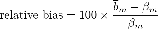
First, at each setting of the experimental conditions, we measured the bias of the sample mediation (difference) coefficient in relative terms as

$\text{relative bias}=\text{1}00\times \frac{{\overline{b}}_m-{\beta }_m}{{\beta }_m}$

where ${\overline{b}}_m$ is the empirical mean of the difference coefficient estimates across the 1,000 replication samples, β_m is the corresponding value of the difference coefficient given by applying the khb routine to each population of N = 10000 synthetic observations for this particular set of experimental conditions, and bias $(b_{\text{m}})={\overline{b}}_m-{\beta }_m$ As noted above, we refer to this criterion as “relative bias”. Second, as an estimate of the random error associated with the difference coefficient estimates from khb, we used the observed (empirical) standard deviation of b_m across the 1,000 replications at each of the experimental conditions, also reported in relative terms here as a percentage of the corresponding β_m . We refer to this in the following as the ESE. Finally, at each of the experimental conditions, we constructed a conventional normal-theory 95% confidence interval of the form $b_m\pm \text{1}.\text{96}{s}_{b_m}$ , where $s_{b_m}$ is the estimate of the standard error of the difference given by khb. For each replication sample, we recorded whether this interval contained the β_m for the parent population, yielding a comparison of actual versus nominal confidence interval coverage across the 1,000 replications. We refer to this criterion as “confidence interval coverage” throughout the analyses.

3.3 Analytical strategy

We used several methods to identify patterns in the criteria listed above. Initially, we present the medians for the three performance criteria broken down by the experimental conditions. We chose medians rather than means to avoid distortions from individual cases where small values for the denominator of the various relative measures led to small absolute errors being enormous in relative terms.

Next, motivated by the complexity of the experimental design, we adopted a regression-based summary of the results to concisely describe how each experimental condition independently affected estimation performance. This regression-based summary gives a more concise and comprehensible description of the results than a tabular summary. Again motivated by some unusual outliers, we used least absolute deviation (LAD) regression, which summarizes how the conditional median of each performance varied across our experimental conditions as opposed to the conditional mean that would result from a conventional (ordinary least-squares) summary.

4 Results

4.1 Tabular analysis

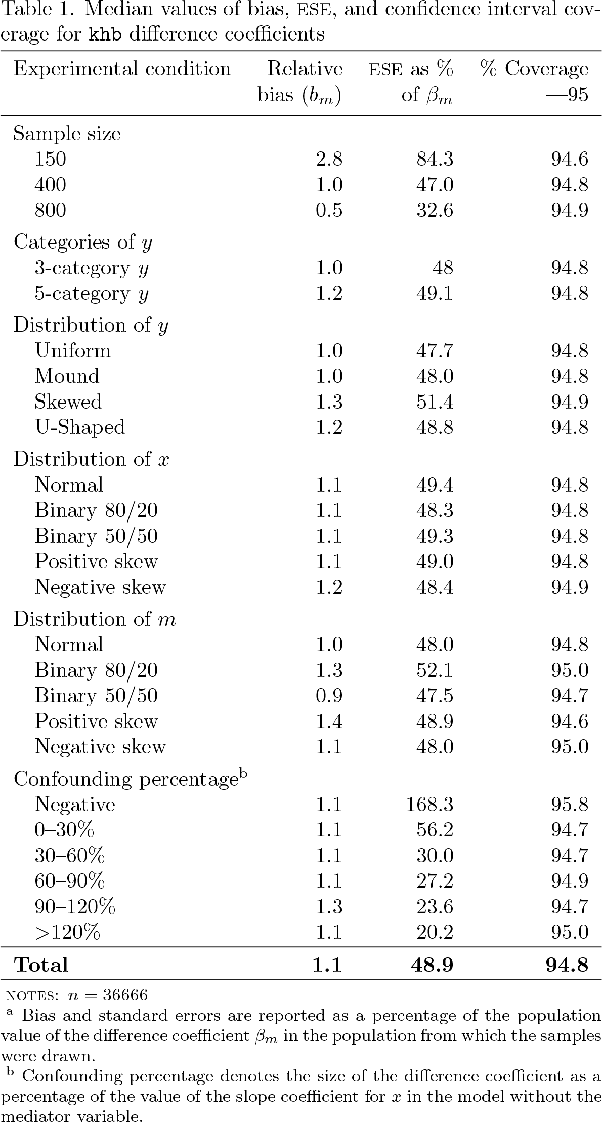
Table 1 displays the median for each performance criterion organized by the experimental conditions. Overall, across all experimental conditions, the b _m difference coefficient showed a slight upward bias with a median relative bias of roughly 1.1% of the population coefficient. The median bias of the b _m was small at all sample sizes but decreased in proportion to 1/N, from 2.8% at n = 150 to 0.5% at n = 800. The median of the relative bias was small across all distributions of the response variable y, as well as across the distributions of x and m and the various confounding percentages, with a range of 0.9% to 1.4% in the median bias across these conditions.

Table 1.

Median values of bias, ESE, and confidence interval coverage for khb difference coefficients

Experimental condition	Relative bias (bm)	ESE as % of βm	% Coverage —95
Sample size
150	2.8	84.3	94.6
400	1.0	47.0	94.8
800	0.5	32.6	94.9
Categories of y
3-category y	1.0	48	94.8
5-category y	1.2	49.1	94.8
Distribution of y
Uniform	1.0	47.7	94.8
Mound	1.0	48.0	94.8
Skewed	1.3	51.4	94.9
U-Shaped	1.2	48.8	94.8
Distribution of x
Normal	1.1	49.4	94.8
Binary 80/20	1.1	48.3	94.8
Binary 50/50	1.1	49.3	94.8
Positive skew	1.1	49.0	94.8
Negative skew	1.2	48.4	94.9
Distribution of m
Normal	1.0	48.0	94.8
Binary 80/20	1.3	52.1	95.0
Binary 50/50	0.9	47.5	94.7
Positive skew	1.4	48.9	94.6
Negative skew	1.1	48.0	95.0
Confounding percentageb
Negative	1.1	168.3	95.8
0–30%	1.1	56.2	94.7
30–60%	1.1	30.0	94.7
60–90%	1.1	27.2	94.9
90–120%	1.3	23.6	94.7
>120%	1.1	20.2	95.0
Total	1.1	48.9	94.8

notes: n = 36666

^a Bias and standard errors are reported as a percentage of the population value of the difference coefficient βm in the population from which the samples were drawn.

^b Confounding percentage denotes the size of the difference coefficient as a percentage of the value of the slope coefficient for x in the model without the mediator variable.

While relative bias was generally quite small, the sampling variability of the estimates, as measured by the ESE as % of β _m, was much larger. The median value of the ESE was 49%, that is, about half as large as the population value of the coefficient being estimated. The ESE varied substantially with the sample size and confounding percentages. First, the median ESE ranged from 84% of the size of the population coefficient at n = 150 to 33% at n = 800, decreasing approximately as 1/√N. Second, the ESE increased substantially as the confounding percentage approached 0%, indicating that estimation becomes more unreliable in relative terms in situations with little mediation. Confidence interval coverage for estimates of the difference coefficient was consistently remarkably good and varied little across any of the experimental conditions with a median of no less than 94.6% (versus the nominal 95%) for any experimental condition.

In summary, our descriptive observations identify relatively limited systematic differences in the performance of khb as a function of sample size, the distribution of y, x, and m, and the confounding percentage. And, more importantly, performance of the khb method appears quite good under nearly all conditions.

4.2 Median regression models

To synthesize the results across multiple experimental conditions, we used LAD regression models to summarize the effect of each condition on the median for each of the performance criteria, displayed in table 2 below. Mirroring the descriptive results, we find that relative bias was largely unaffected by any experimental condition except sample size at n = 150 because no other conditions affected relative bias by more than about 0.5 percentage points. Compared with n = 800, the relative bias increased by roughly 2.4 percentage points when n = 150 and 0.5 percentage points when n = 400. Other relatively small but notable differences were observed between the number of categories and distributions y, as well as the distribution of m, but not x. In sum, the model suggests little bias in estimation of the difference coefficient.

Table 2.

Coefficients (standard errors) from LAD regression^a models for khb measures as a function of experimental conditions

	Relative bias (b m)b	ESE as % of β m c	% Coverage—95d
Sample size (ref. n = 800)
n = 150	2.35**	50.53**	−0.35**
	(0.03)	(0.34)	(0.02)
n = 400	0.52**	15.73**	−0.10**
	(0.03)	(0.34)	(0.02)
y categories (ref. 5-categories)
3-categories	0.21**	0.35	−0.00
	(0.02)	(0.28)	(0.02)
y distribution (ref. y = mound)
Uniform	0.00	0.26	0.00
	(0.03)	(0.40)	(0.02)
Skew	0.50**	2.79**	0.05*
	(0.03)	(0.40)	(0.02)
U-Shaped	0.23**	0.75	0.00
	(0.03)	(0.40)	(0.02)
x distribution (ref. x = normal)
80/20	−0.04	0.36	0.00
	(0.04)	(0.45)	(0.03)
50/50	−0.03	−0.40	−0.00
	(0.03)	(0.44)	(0.03)
Positive skew	0.01	0.20	−0.00
	(0.03)	(0.44)	(0.03)
Negative skew	0.11**	−0.01	0.10**
	(0.03)	(0.44)	(0.03)
m distribution (ref. m = normal)
Positive skew	0.35**	2.75**	0.25**
	(0.04)	(0.45)	(0.03)
Negative skew	−0.13**	−0.27	−0.05
	(0.03)	(0.44)	(0.03)
50/50	0.40**	1.19**	−0.20**
	(0.03)	(0.44)	(0.03)
80/20	0.10**	−0.07	0.25**
	(0.03)	(0.44)	(0.03)
Confounding %	0.02	−50.93**	0.00
Constant	(0.03)	(0.44)	(0.03)
	0.09*	43.93**	94.85**
N	36,666	36,666	36,666

notes: * p < 0.05; ** p < 0.01

^a All estimates here are from absolute-deviation (median) regression models. Table entries are therefore slopes of the conditional median with respect to each experimental condition variable.

^b Bias of the difference coefficient as a percentage of its population value.

^c ESE of the difference coefficient as a percentage of its population value.

^d Percent of time-asymptotic confidence interval included the population value of the difference coefficient.

Results for the second LAD model showed that the ESE as % of β _m was sensitive to sample size, with the median ESE being about 50 percentage points higher at n = 150 than at n = 800 and 15 percentage points higher at n = 400, controlling for all other conditions. Further, the ESE was substantially larger at smaller confounding percentages. To better understand this relationship, we conducted a supplementary analysis, predicting values of the ESE by confounding percentage, with results shown graphically in figure 1 below. Our model predicts that the ESE as a percentage of the population coefficient is roughly 70% when the confounding percentage is near zero, but the empirical standard decreases dramatically as the confounding percentage increases. This is again unsurprising because these results at least partially reflect the small denominator value of the difference coefficient in these relative measures. Finally, the predicted ESE was largely unaffected by the number of categories of the response variable y or the distributions of x and m.

Figure 1.

Predicted value of ESE as % of β _m by confounding percentage

Finally, we found that under all experimental conditions, confidence interval coverage did not vary more than 0.5 percentage points from the median. Again, sample size was the largest source of differentiation, where in comparison with n = 800, confidence interval coverage is 0.4 percentage points less at n = 150 and 0.1 percentage points less at n = 400. Further, confidence interval coverage was largely unaffected by the number of categories of y, or the distribution of y or x, but was partially influenced by distributions of m. Compared with a normally distributed m, distributions with a positive skew and 80/20 binary split are 0.3 percentage points higher in confidence interval coverage, while conversely the coverage was 0.2 percentage points lower for 50/50 binary splits. Confounding percentage also appears to have no effect on the confidence interval coverage. As such, we observe that under all conditions, the khb estimate of the difference coefficient’s 95% confidence interval generally contains the population parameter.

5 Discussion and conclusion

The khb method of adopting difference coefficients to estimate the amount of mediation (confounding) solves the well-known and long-standing issues associated with conducting mediation analysis in nonlinear models. In the preceding analyses, we exhaustively evaluated the performance of the khb technique for estimating mediation in nonlinear response models, using ordinal logistic regression as an exemplar.

While we do not comment on the underlying theory of how best to measure mediation, we can confidently argue that—at least for the ordinal response models analyzed here—the estimation performance of these measures is excellent as judged by bias in the estimation of the difference coefficient, even at small-sample sizes, and actual confidence interval coverage closely matched nominal values.

Our analysis goes substantially beyond previous analyses (see Karlson and Holm [2011]; Best and Wolf [2012])—which used a large-sample size and focused on binary outcomes—and provides a more rigorous and comprehensive understanding of the khb technique. We expanded upon these previous analyses in four key ways: First, we analyzed the performance of khb with regard to ordinal response models, building upon previous work that had included only binary response models (see Karlson and Holm [2011]; Karlson, Holm, and Breen [2012]; Best and Wolf [2012]). Second—and related to the first point—estimation of ordinal models, while unique, could also present a more difficult case for the khb method. Third, previous performance analyses have focused solely on the mediation coefficient, while this analysis also paid attention to its variance. Finally, we provided a far broader, and arguably more difficult, range of simulation conditions than assessed in previous studies.

Our results show that khb performs remarkably well in many scenarios for ordinal outcomes. While we have discussed conditions under which khb‘s performance degrades, we suggest that overall khb estimates the difference coefficient with modest biases. But the estimation of the standard error is comparatively more troublesome with greater observed relative biases. This finding on the difficulty of estimating standard errors is in line with previous studies of binary logistic regression, where the bias of the sample variance of slope estimates is commonly larger than the bias of the slope estimates themselves (see Nemes et al. [2009]; Pawitan [2001]).

Further, confidence interval coverage is quite accurate, with an average coverage of 94.7% across all simulations versus the nominal level of 95%. Sample size is a strong, consistent predictor of bias in the estimation of the difference coefficient and ESE, but even in the worst case of n = 150, khb performs well. Overall, our results suggest that researchers using khb can assume that it reasonably approximates parameters.