gidm: A command for generalized inflated discrete models

Abstract

In this article, we describe the gidm command for fitting generalized inflated discrete models that deal with multiple inflated values in a distribution. Based on the work of Cai, Xia, and Zhou (Forthcoming, Sociological Methods & Research: Generalized inflated discrete models: A strategy to work with multimodal discrete distributions), generalized inflated discrete models are fit via maximum likelihood estimation. Specifically, the gidm command fits Poisson, negative binomial, multinomial, and ordered outcomes with more than one inflated value. We illustrate this command through examples for count and categorical outcomes.

1 Introduction

Social science researchers have long recognized the inflation of certain values for discrete variables. For example, the number of children born within a family is concentrated on values of 0, 1, and 2 (Poston and McKibben 2003). Inflation brings challenges to traditional discrete models. For instance, the observed proportions for the inflated values exceed the probabilities that regular distributions would allow. If not modeled properly, inflations might lead to biased estimates and incorrect inferences (Lambert 1992).

Past decades have witnessed a rapid development of inflated models. Scholars have extended the inflation models not only on the forms of discrete distributions but also on allowing the number of inflation points to be more than one. To address an excess of zero counts in data, Lambert (1992) proposed a zero-inflated Poisson (ZIP) model that implements two separate models—a Poisson count model and a logit model for predicting excessive zeros. In the same vein, the zero-inflated framework has been applied to other discrete distributions, such as zero-inflated negative binomial (ZINB) regression (Ridout, Hinde, and Dem´eAtrio 2001); the zero-inflated binomial model (Diop, Diop, and Dupuy 2016; Hall 2000; Vieira, Hinde, and Demetrio 2000); zero-inflated multinomial regression (Diallo, Diop, and Dupuy 2018); the inflated ordered logistic model (Bagozzi and Mukherjee 2012); and the zero-inflated ordered probit (ZIOP) model (Bagozzi et al. 2015).

Recently, scholars have extended the zero-inflated models to allow for an arbitrary number of inflation points. For example, Lin and Tsai (2013) proposed a zero-k-inflated Poisson model that allows a second inflation point at the value k besides zero. Begum, Mallick, and Pal (2014) suggested a generalized inflated Poisson (GIP) model to address multiple inflations for responses in categorical forms. The most recent work by Cai, Xia, and Zhou (Forthcoming) has further extended GIP to a general form and introduced a generalized inflated discrete model (GIDM), which uses arbitrary and multiple inflations for a wide range of discrete probability distributions, such as multinomial, ordinal, Poisson, and zero truncated Poisson.

Despite the recent theoretical development of inflated models, the implementation has been lacking, especially for Stata users. Prior to Stata 15, zip and zinb were the only two available commands for modeling zero-inflated counts. Stata 15 introduced the ZIOP model via the command zioprobit. To the best of our knowledge, GIDM has not been integrated into Stata. To fill this gap, we developed the gidm command to implement the GIDMs, including the GIP, generalized inflated negative binomial, generalized inflated multinomial, and generalized inflated ordered models.

The rest of this article is organized as follows: Section 2 gives a brief introduction of GIDM, focusing on estimation. Section 3 explains the syntax and options of the gidm command. Sections 4 and 5 present illustrations using two well-known examples: the number of fish caught in a state park and the fictional data on smoking habits. Section 6 discusses issues such as the goodness of fit, nonconvergence problems, and further directions of development.

2 The GIDM

Following Begum, Mallick, and Pal (2014), Cai, Xia, and Zhou (Forthcoming) suggested a general framework of inflated values for discrete outcomes. Suppose Y is a discrete random variable that has inflated probabilities at values k ₁ ,…, k_m ∊ {0, 1, 2,…}. The probability mass function (PMF) could be written as

$p(Y=k|\lambda ,{\pi }_i,1\le i\le m)=\{{ }_{(1-{\displaystyle \sum { }_{i=1}^m}{\pi }_i)\times p(k|\lambda ) \text{if}\hspace{0.17em}k\ne k_i,1\le i\le m}^{{\pi }_i+(1-{\displaystyle \sum { }_{i=1}^m{\pi }_i)}\times p(k|\lambda ) \text{if }k=k_1,\mathrm{...},k_m}$

where p(Y = k|λ) is a discrete PMF with the parameter λ for outcome k, π_i is the probability of inflation at the value k_i with 1 ≤ i ≤ m, and ${\displaystyle {\sum }_{i=1}^m{\pi }_i\in (0,1)}$ .

The above parameterization suggests that the PMF can be considered a combination of probabilities for several binary outcomes and one regular discrete outcome. If the value k_i for a respondent falls in the set of inflated values k ₁ ,…, k_m ∊ {0, 1, 2,…}, the PMF is a sum of two components: π_i denoting the chance of inflation for value k_i and $(1-{\displaystyle {\sum }_{i=1}^m{\pi }_i})\times p(k_i|\lambda )$ indicating the conditional probability for value k_i from the regular discrete PMF, for example, Poisson, negative binomial, etc. If k_i does not belong to the set of inflated values, the PMF shrinks to the conditional probability of $(1-{\displaystyle {\sum }_{i=1}^m{\pi }_i})\times p(k_i|\lambda )$ . The probability of inflation at the value k_i , π_i could also depend on covariates. For example, if a logit model is specified,

${\pi }_i=\frac{1}{1+\exp (-z_s{\gamma }_i)}$

where z_s and γ_i is the vector of predictors for the sth observation and the vector of corresponding parameters, respectively. A probit model could be derived if a probit function is specified for π_i .

The GIDM offers a framework that covers all the inflated models commonly seen in social sciences, such as ZIP, ZINB, GIP, generalized inflated negative binomial, generalized inflated multinomial, and generalized inflated ordered. Once the GIDM is specified, the full likelihood function L(θ) can be constructed accordingly. The maximum likelihood estimator of the unknown parameter of θ can be obtained by solving the score function:

$\frac{\delta \log L(\theta )}{\delta \theta }=0$

The Fisher information matrix can be obtained by taking the second derivative of the log likelihood with respect to θ. The unknown parameters θ can be estimated by method of moments (Hansen 1982), direct maximum likelihood (Cai, Xia, and Zhou Forthcoming), or maximum likelihood via the expectation-maximization algorithm (Begum, Mallick, and Pal 2014). Diallo, Diop, and Dupuy (2018) provided a rigorous investigation of the maximum likelihood estimator in terms of the identifiability, existence, consistency, and asymptotic normality under classical regularity conditions.

The gidm command maximizes the log likelihood of GIDM using Stata’s ml command (Gould, Pitblado, and Poi 2010). The gidm command supports the specification of the following distributions: Poisson, negative binomial, ordinal logistic and probit, and multinomial logistic and probit. Binomial distribution is not singled out in the gidm command, because it can be estimated as a two-category case of multinomial distribution.

3 The gidm command

3.1 Description

The gidm command fits a GIDM of depvar on several sets of indepvars and varlistN. The depvar is a nonnegative integer of the response variable. The indepvars is a set of explanatory variables for depvar, whereas varlist1 to varlistN are sets of explanatory variables for modeling the probabilities of inflation at each of the points corresponding to the values specified in the numlist in the option inflation( numlist ). Specifically, an intercept-only model can be specified as (_con).

3.2 Syntax

gidm (depvar indepvars) (varlist1) […(varlistN)] [if] [in] [weight] , inflation(numlist) link(string) [noinitial vce(vcetype) level(#) display_options maximize options]

3.3 Options

inflation( numlist ) specifies the list of values at which the inflations are assumed. The number of elements in numlist must be the same as the number of equations specified by indepvars and varlist1…varlistN. inflation() is required.

link( string ) defines the distribution for both of the noninflated and the inflated parts. We use a four-letter combination to represent each model. The first two letters, for example, lg for logit and pb for probit, indicate the functional form for the inflated part, and the last two letters refer to the distribution of outcome. The supported distributions for the outcome are Poisson (po), negative binomial (nb), multinomial (ml), cumulative logit (cl), and cumulative probit (cp). For instance, the keyword lgpo refers to a logit-inflated Poisson, and pbcp is a probit-inflated cumulative probit. link() is required. A summary of the keywords of models supported by the gidm command is given in table 1.

Table 1.

Link options

Outcome	Model	Option link(string)
		Logit inflations	Probit inflations
Count	Poisson	lgpo	pbpo
	Negative binomial	lgnb	pbnb
Category	Multinomial	lgml	pbml
	Ordered logit	lgcl	pbcl
	Ordered probit	lgcp	pbcp

noinitial suppresses the default initial values that are from results of the separately fit model parts. For example, with link(lgpo), the default initial values are obtained from a separately fit Poisson model for the main part and logistic regressions for the inflated parts.

vce( vcetype ) specifies the type of standard error reported, which includes types that are derived from asymptotic theory (oim, opg), that are robust to some kinds of misspecification (robust), that allow for intragroup correlation (cluster clustvar), and that use bootstrap or jackknife methods (bootstrap, jackknife); see [R] vce option.

level( # ); see [R] Estimation options.

display options: noci, nopv alues, noomit ted, vsquish, noempty cells, base levels, allbase levels, nofvlab el, fvwrap( # ), fvwrapon( style ), cformat(% fmt ), pformat(% fmt ), sformat(% fmt ), and nolstretch; see [R] Estimation options.

maximize options: dif ficult, tech nique(algorithm spec), iter ate(# ), no lo g, tr ace, grad ient, showstep, hess ian, showtol erance, tol erance(# ), ltol erance(# ), nrtol erance(# ), nonrtolerance, and from( init specs ); see [R] Maximize. These options are seldom used.

Setting the optimization type to technique(bhhh) resets the default vcetype to vce(opg).

3.4 Stored results

gidm stores the following in e():

4 The number of fish caught example: The inflated count models

The number of fish caught dataset is used to showcase the capability of the gidm command for fitting inflated count models. The dependent variable is the number of fish caught for each individual (count). The independent variables include whether the individuals brought a camper (camper), how many adult people were in the group (persons), and how many children were in the group (child). Figure 1 shows that there are large proportions of visitors who did not harvest any fish (56.8%), or only one (12.4%), although the average number of fish caught was 3.296.

Figure 1.

Histogram of fish count

We first run Stata’s zip command with the variables child and camper as the predictors for the number of fish caught. The variable persons is set as the only predictor for the probability of inflation—the excess zeros. Then, the same model is fit using the gidm command. Notice that the zip command specifies the dependent variable and the predictors of the Poisson part in the main part of the command and uses the option inflate() to specify variables that predict the inflation. The gidm command allows users to specify the predictors of both the Poisson and the inflated parts in the main body and separates them by parentheses for the Poisson part and the inflated part. Two options, inflation() and link(), are used to define the value at which inflation is assumed and the distribution of outcome, respectively.

Comparing the estimates obtained from the two commands, we see that the coefficients, the standard errors, the p-values, and the confidence intervals are the same past the fourth decimal place. If a ZINB model is specified, the gidm command generates the same estimates, standard errors, and p-values compared with those obtained from the zinb command, although the latter outputs more information. Users can get exponentiated coefficients and a description of the dependent variable. Thus, the gidm command provides a convenient and integrated alternative to estimate both ZIP and ZINB models.

Including extra inflation points is straightforward—by adding sets of predictors in the main part of the command and specifying additional inflation points in the inflation() option. For example, a zero-one-inflated Poisson model (Melkersson and Olsson 1999) can be specified as follows:

The results indicate that the number of people contributes not only to the inflation at value 0 but also to that at value 1. The more people in a group, the less likely the number of fish caught will be 0 or 1.

5 The tobacco example: The inflated cumulative probit and logit models

We use the tobacco data to show how to implement the inflated ordered logistic and probit models. Suppose we are interested in factors that contribute to the number of cigarettes smoked per day by an individual. The dependent variable tobacco measures the number of cigarettes smoked in a day and has been grouped into four levels: 0 cigarettes, 1 to 7 cigarettes/day, 8 to 12 cigarettes/day, and more than 12 cigarettes/day coded as 0, 1, 2, and 3, accordingly. The independent variables included are female, income, and age. Usually, the natural choice for the ordered outcomes is either an ordered logistic or a probit model with a proportional odds assumption, which assumes that the effects of independent variables are the same for different levels of responses and that the only difference lies in the intercepts and thresholds. Because the descriptive statistics show that 63.1% of respondents were nonsmokers, it is reasonable to assume a zero-inflated model with probit or logit for the inflation part. We use both the command gidm and the Stata command zioprobit to fit a ZIOP. Besides the independent variables, two additional variables—whether a parent smoked (smoking) and whether a respondent’s religion discourages smoking (religion)—are also enclosed to account for the inflation on zeros. The output below shows that the results obtained from both commands are identical.

Stata does not have a command to fit a zero-inflated ordered logistic model; however, it can be easily done in the command gidm by changing the string of the link( string ) option to lgcl as follows.

The results from the ZIOP and zero-inflated ordered logistic models suggest that the income is positively associated with tobacco use, while age and gender are negatively correlated. Furthermore, with smoking parents, one is expected to more likely be a smoker or less likely be a nonsmoker. Interestingly, the effect of income is two-fold: income increases the chance to be a nonsmoker; while once started smoking, higher income is correlated to more cigarettes consumed per day.

Because of different parameterization, the sign of coefficients using a probit link is opposite to that using a logit link, although the size of coefficients is very close (Moore 2013). As a simple illustration, we can extend the inflation part to include the value 1 to see whether age contributes to light smoking by using a logit link. According to the result below, age also reduces the chance of inflation at the category of 1 to 7 cigarettes/day.

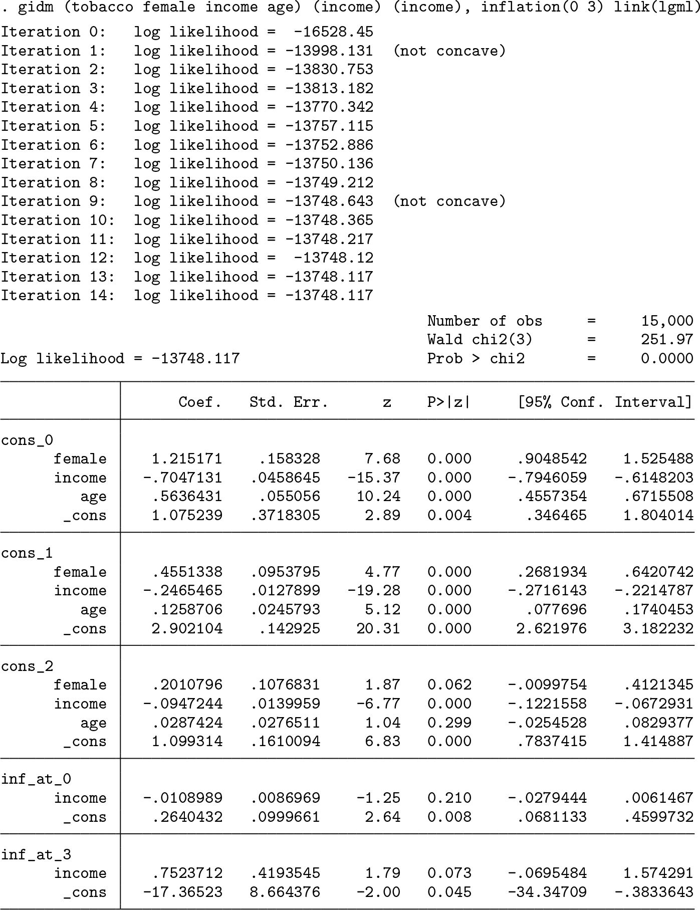
One may wonder what if the proportional odds assumption does not hold, for example, the effects of independent variables vary by categories of the dependent variable. We can fit an inflated multinomial logit or probit model by changing the string of the link( string ) option to lgml or pbml, respectively. The output is as follows.

Based on the results from both models, the effects of independent variables do vary across the categories with respect to the reference group. For instance, with respect to the reference category, the effect size of income reduces (for example, −0.705 versus −0.247 versus −0.095), while the category of frequency of smoking increases. Note that the estimated standard error of the intercept for inflation at 3 is large, although the z test reaches significance at the conventional 5% level, which is a sign that the inflation at 3 might not exist. In sum, the gidm command offers a flexible parameterization that allows for multiple inflated values as well as link functions.

6 Discussion

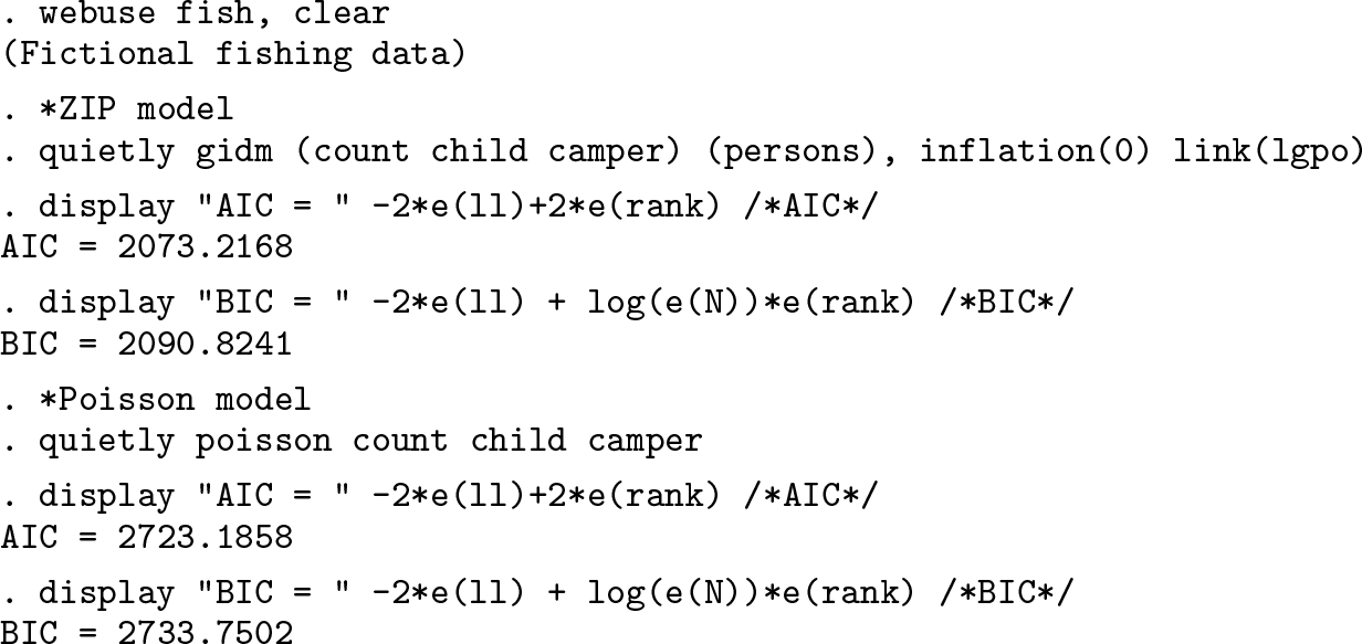
Traditionally, the Vuong (1989) test is used to evaluate goodness of fit for the inflated models. However, a recent study suggests that the Vuong test is not appropriate for testing possible inflation (Wilson 2015). Because Stata 15 removed the Vuong test from their zip, zinb, and zioprobit commands, ¹ in the current study, we use only the Akaike information criterion (AIC) and Bayesian information criterion (BIC) as criteria to compare the goodness of fit across models. For instance, in the number of fish caught example, the AIC and BIC for the inflated and the regular models can be calculated as follows.

The values of the AIC and BIC for the ZIP model are much lower than that of the regular Poisson, which indicates the ZIP fits the data better.

When one optimizes the likelihood function of the GIDM, most of the models implemented in the gidm command require only lf0 or lf1 (Gould, Pitblado, and Poi 2010) to converge. However, sometimes numerical issues such as nonconvergence, or overflow, may occur if the empirical derivatives of the likelihood function are hard to evaluate numerically. The most common explanation for the numerical issues might be model misspecification, especially for the inflation part. Users should be cautious about the number of values and predictors enclosed for the inflation part. It is helpful to start with a simple model, for example, intercept only for the inflation part, and then build upon it.

If the model is correctly specified, one way to improve numerical stability is to fit the model using lf2 (Gould, Pitblado, and Poi 2010). Although it is feasible, the Hessian matrix may still be expensive or cumbersome to evaluate; for instance, the computational recourses required for calculating the second derivative for an ordinal or multinomial outcome with multiple inflations might be large. An alternative is to replace the gradient or Hessian with less expensive approximations. For instance, suppose a multinomial random variable Y has inflated probabilities at categories k ₁ ,…, k_m ∊ {0, 1, 2,…}; the PMF for each of the observations could be written as

$p(Y=k|{\beta }_k,{\pi }_i,1\le i\le m)=\{{ }_{(1-{\displaystyle \sum { }_{i=1}^m}{\pi }_i)\times p(k) if\hspace{0.17em}k\ne k_i,1\le i\le m}^{{\pi }_i+(1-{\displaystyle \sum { }_{i=1}^m}{\pi }_i)\times p(k) i\text{f}\hspace{0.17em}k=k_1,\mathrm{...}{k}_m}$

where $p(k)=pk=\{\exp (x_s{\beta }_k)\}/\{1+{\displaystyle \sum { }_{k=1}^K}\exp (x_s{\beta }_k)\}$ , $pk=1-{\displaystyle \sum { }_{k=1}^{K-1}}pk$ , and π_i = 1{1 + exp(−z _s γi)}. If we define the indicator as J_i := 1 _{k =k} 1 _,…,k m, then the log likelihood is

$\log L={\displaystyle \sum _{k=1}^K\left({ }_{(1-J_i)\times I(y_s=k)\times \{\log (1-{\displaystyle \sum { }_{i=1}^m}{\pi }_i)+\log (p_k)\}}^{J_i\times I(y_s=k)\times \log \{{\pi }_i+(1-{\displaystyle \sum { }_{i=1}^m}{\pi }_i)\times pk\}+}\right)+c}$

The first derivative with respect to p_j is as follows.

$\frac{\partial \log L}{\partial p_j}={\displaystyle \sum _{k=1}^K\left({ }_{(1-J_i)\times I(y_s=k)\times \left(\frac{1}{p_k}\frac{\partial p_k}{\partial p_j}\right)}^{J_i\times I(y_s=k)\times \frac{1-{\displaystyle \sum { }_{i=1}^m}{\pi }_i}{{\pi }_i+(1-{\displaystyle \sum { }_{i=1}^m}{\pi }_i)\times p_k}\frac{\partial p_k}{\partial p_j}+}\right)}$

Because the term

$\frac{1-{\displaystyle \sum { }_{i=1}^m}{\pi }_i}{{\pi }_i+(1-{\displaystyle \sum { }_{i=1}^m}{\pi }_i)\times p_k}=\frac{1}{\frac{{\pi }_i}{1-{\displaystyle \sum { }_{i=1}^m}{\pi }_i}+pk}\le \frac{1}{pk}$

then

$\frac{\partial \log L}{\partial P_j}\le {\displaystyle \sum _{k=1}^K\left\{I(y_s=k)\times \frac{1}{pk}\frac{\partial pk}{\partial pj}\right\}}$

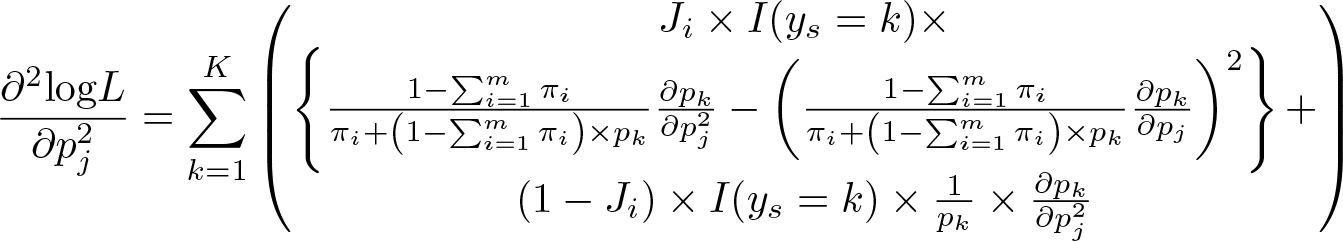
It reaches to equality if π_i is zero. Thus, a majorization of the first derivative can be derived. If we look further, the diagonal elements of the second derivative yield

$\frac{\partial \log L}{\partial P_j}={\displaystyle \sum _{k=1}^K\left(\begin{array}{c}{J}_i\times I(y_s=k)\times \\ \left\{\frac{1-{\displaystyle \sum { }_{i=1}^m}{\pi }_i}{{\pi }_i+(1-{\displaystyle \sum { }_{i=1}^m}{\pi }_i)\times p_k}\frac{\partial pk}{\partial p_j^2}-{\left(\frac{1-{\displaystyle \sum { }_{i=1}^m}{\pi }_i}{{\pi }_i+(1-{\displaystyle \sum { }_{i=1}^m}{\pi }_i)\times p_k}\frac{\partial p_k}{\partial p_j}\right)}^2\right\}+\\ (1-J_i)\times (y_s=k)\times \frac{1}{p_k}\times \frac{\partial p_k}{\partial p_j^2}\end{array}\right)}$

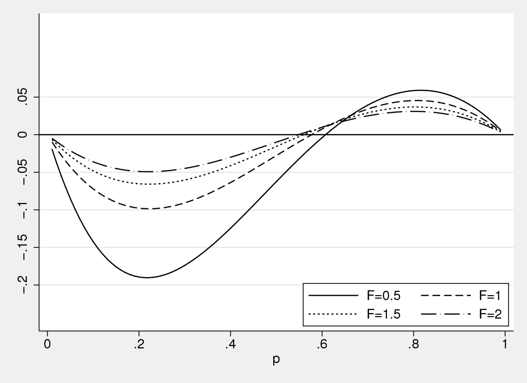
However, (∂ ²logL)/(∂pj ²) is negative only if p_k < (1/2). If p_k ≥ (1/2), the Hessian might not be positive definite. Therefore, it is necessary to check model specification to make sure that p_k < (1/2). If we define the inflation factor as $F={\pi }_i/(1-{\displaystyle \sum { }_{i=1}^m}{\pi }_i)$ , figure 2 summarizes the relationship between the size of the inflation factor and the second derivative. Numerical issues may emerge if the inflation factor is small and the probability p_i is large. In other words, if data show a high percentage for one category, but the relative chance of inflation for that category is small, the model is likely to have nonconverge issues.

Figure 2.

Relationship between the inflation factor and the second derivative

According to our experiment, even under a mild or severe situation, for example, the percentage of p_k ≥ (1/2) is higher than 65%, all three methods, lf0, lf1, and lf2, yield reasonable estimates, with a convergence rate of about 90%, especially for the lf1 method, which requires fewer numbers of iterations and Hessian calls.

The current implementation can be further extended in several ways. A direct extension is to allow for continuous or truncated outcomes such as linear or zero-truncated models. Another useful extension might be to support predictions after estimation. At present, we are working on adding predictions, residuals, influence statistics, and the like. In addition, although the option vce() offers robust standard errors to account for clustering, a more efficient method would be to allow random effects. Therefore, future work will also cover random- and fixed-effects models.

Nevertheless, the GIDM framework is a powerful tool for analyzing inflated outcomes. Despite the recent development of the generalized inflation models, the modeling choices for Stata users are limited. We developed the gidm command, which supports various distributions, to fit the most recent version of the inflated models—the GIDM. Meanwhile, the traditional single-value inflated models are also available as special cases in the gidm command. We hope the gidm command developed in this article will be useful for Stata users when dealing with inflation problems.

Supplemental Material

Supplemental Material, st0574 - gidm: A command for generalized inflated discrete models

Supplemental Material, st0574 for gidm: A command for generalized inflated discrete models by Yiwei Xia, Yisu Zhou and Tianji Cai in The Stata Journal