Sage Journals: Discover world-class research

Abstract

In this article, I describe a community-contributed command, intcount, that fits one of several regression models for count data observed in interval form. The models available are Poisson, negative binomial, and binomial, and they can be fit in standard or zero-inflated form. I illustrate the command with an application to analysis of data from the UK Understanding Society survey on the demand for healthcare services.

Keywords

st0571 intcount count data interval data zero-inflated interpolation Understanding Society

1 Introduction

Many survey variables are naturally nonnegative integer-valued counts, for example, the number of times an action or event has occurred within a given observation period. Count-data regression models based on distributions, such as the Poisson and negative binomial models, are widely used to analyze these variables.

But complications arise when survey questions are not designed to reveal the count exactly. Survey designers sometimes argue that questions may yield more reliable (albeit less detailed) data if they ask the respondent to place the count within one of a number of prespecified intervals, rather than to report a specific figure.

Interval observation of count data causes difficulty in the estimation of count-data regressions, because most available software requires the count to be observed exactly. Therefore, there is a need for estimation procedures that can account for coarse interval observation.¹ Furthermore, many types of descriptive or policy analysis require exact rather than interval counts, so some form of imputation or interpolation is required.

In this article, I describe a new command for interval estimation of a number of count-data models, and I report results from an illustrative application. Section 2 sets out the estimation approach and the range of available models. Section 3 details the syntax of intcount and the linked predict command that can be used for various types of postestimation imputation. Section 4 presents an application to healthcare data from the UK Understanding Society survey. Section 5 concludes.

2 Interval-observed count-data models

2.1 Basic setup

Let Y_i ≥ 0 be the ith observation on a dependent variable that takes nonnegative integer values. Y_i may be bounded or unbounded. However, our observations are not on Y_i itself but rather an interval in which Y_i lies. Consequently, we have two observed dependent variables, [L_i, U_i], with the property that

L_{i} \leq Y_{i} \leq U_{i}

The numerical values of the interval bounds [L_i, U_i] vary across observations, but they are assumed to be observed and strictly exogenous. The two bounds may be equal for some observations where Y_i is fully observed, and, for unbounded distributions like the Poisson and negative binomial, the upper bound U_i may be infinite for some observations.

A set of explanatory covariates appears in a vector X _i , and we assume a known parametric form for the discrete conditional probability function f(·) and corresponding distribution function F (·), defined for any nonnegative integer y:

\begin{matrix} P r (Y_{i} = y | X_{i}) = f (y | X_{i}) \\ P r (Y_{i} \leq y | X_{i}) = F (y | X_{i}) \end{matrix}

The conditional probability of observing the event L_i ≤ Y_i ≤ U_i is

\begin{array}{l} Pr (L_{i} \leq Y_{i} \leq U_{i} | X_{i}) = F (U_{i} | X_{i}) - F (L_{i} - 1 | X_{i}) \\ = \sum_{y = L_{i}}^{U_{i}} f (y | X_{i}) \end{array}

where F (L_i − 1| X _i ) is understood to be zero for L_i = 0.

2.2 Alternative base distributions

The model is completed by specifying a parameterized functional form for the distribution function F (·| X _i ). The command offers nine possibilities formed from three alternative base models and three options for zero inflation. If we leave aside the possibility of zero inflation, the available models for F (·| X _i ) are as follows:

The Poisson model is

f (y | X_{i}) = e^{- λ_{i}} λ_{i}^{y} / y!

where λ_i is the conditional mean function E (Y_i| X _i ) parameterized as e^Xi^β. The conditional mean and variance of the count variable are both equal to λ_i.

The binomial model is

f (y | X_{i}) = (\begin{array}{l} M_{i} \\ y \end{array}) p_{i}^{y} {(1 - p_{i})}^{M_{i} - y}

where M_i is the known maximum possible value, which may vary exogenously across observations, and p_i is the binomial probability, parameterized as p_i = (1 − e⁻ ^X i^β)⁻¹. The conditional mean function is E (Y_i| X _i ) = M_ip_i. This specification may be appropriate when there is a natural upper limit to survey responses (for example, to the question “on how many days last month did you use cannabis?”).

The negative binomial model is derivable as the Poisson-gamma mixture

y | ν \sim Poisson (λ_{i} ν) ν \sim gamma (\frac{1}{α}, α)

where λ_i = e^Xi^β, α > 0. This gives a distribution for y with mean λ_i and variance 1 + αλ_i. Note that, in the terminology of Cameron and Trivedi (2013), this is the NB2 parameterization of the negative binomial regression model and is consistent with the specification implemented in the Stata zinb command. The ML estimation procedure treats ln α as an unrestricted constant parameter.

2.3 Zero inflation

In some count-data applications, standard forms like the binomial, Poisson, and negative binomial are found to understate the frequency of zero counts. One way of dealing with this is to use a double hurdle or mixture process, where some individuals have a degenerate zero count with probability 1, while others have a count drawn from a standard distribution such as the Poisson.

Let the conditional probability of a degenerate zero be given by the linear index model

Pr(degenerate 0 | X_{i}) = π (X_{i 1} γ)

where X _i ₁ is a subvector of X _i . The distribution of Y among the nondegenerate population is g(y| X _i ₂β), where X _i ₂ is another subvector of X _i . Then the mixture distribution of Y is

f (y | X_{i}) = {\begin{cases} π (X_{i 1} γ) + {1 - π (X_{i 1} γ)} g (0 | X_{i 2} β) if y = 0 \\ {1 - π (X_{i 1} γ)} g (y | X_{i 2} β) if y > 0 \end{cases}

The probability of the observed interval [L_i, U_i] is again given by (1).

The intcount command offers three options for zero inflation:

standard model: π( X _i ₁γ) = 0

logit: π( X _i ₁γ) = {1 + exp(− X _i ₁γ)}⁻¹

probit: π( X _i ₁γ) = Φ( X _i ₁γ)

In practice, estimates of the logit and probit variants are usually almost identical apart from scaling of the γ coefficients, which are larger by a factor of approximately $π / \sqrt{3}$ .

2.4 Estimation

Estimation is by maximum likelihood (ML), with probabilities of the form (1) used to construct the log-likelihood function. By default, numerical optimization of the log likelihood is carried out using Stata’s modified Newton–Raphson optimizer; other algorithms can be substituted if you have difficulty in obtaining convergence (see StataCorp [2017, 639–686] for details). Optimization is based on the lf0 evaluator, so log-likelihood derivatives are approximated by finite differences.

Experience to date suggests that this works well in most cases. Difficulties are most likely to be encountered with overspecified models involving zero inflation that is not required by the data, in which case one or more parameters in the coefficient vector γ will explode. Similar convergence Difficulties may be found also in zero-inflated specifications where zero inflation is required empirically for a group with certain values for the variables X _i ₂ but not for other sample groups. These convergence problems are usually easy to spot, and the required model respecification is obvious.

Occasionally (usually in the more heavily parameterized zero-inflated specifications), the optimizer reaches a difficult region with almost flat likelihood or discontinuous approximate derivatives. Often, these problems can be resolved by passing down the estimates from a simpler specification as starting values for the optimization—for example, a model without zero inflation or with constant zero inflation or a Poisson model as a simpler alternative to the negative binomial.

2.5 Prediction and imputation

The estimates provided by intcount may often be useful for imputation, and the predict command available with intcount offers options. Particularly useful options are the interval-conditional mean predictor $Y_{i}^{*} = E (Y_{i} | L_{i} \leq Y_{i} \leq U_{i,} X_{i})$ and the interval-conditional random draw, $Y_{i}^{+}$ , which is a realization of the distribution of Y_i|L_i ≤ Y_i ≤ U_i, X _i . Two common situations illustrate their use.

One is where we would like to use the unobserved variable Y_i as a covariate in another model—for example, a regression of some dependent variable W_i on Y_i and X _i . But Y_i is unobserved, and we know only that it lies within an interval [L_i, U_i]. Then intcount can be used to fit a count-data model for Y_i on X _i and compute the interval-conditional mean predictor $Y_{i}^{*}$ . The use of $Y_{i}^{*}$ as a proxy for Y_i introduces an imputation error proportional to $(Y_{i} - Y_{i}^{*})$ into the regression residual term, but it is straightforward to show that $E {(Y_{i} - Y_{i}^{*}) | Y_{i}^{*}, X_{i}}$ E{(Y_i − Yi^∗)|Yi^∗, X _i } = 0, so the residual is orthogonal to the constructed proxy for Y_i, and the regression of W_i on Y_i, X _i therefore gives unbiased coefficients under standard classical assumptions (provided the count-data model for Y_i| X _i is well specified). This is a better solution to the imputation problem than the common practice of using interval midpoints. However, it can be improved further by making random draws Yi+ and using single or multiple imputation.²

Another common application is where exact values for Y are needed within some complex policy simulation. Again, multiple random draws Yi+ can be used in place of the unobserved Y_i, and the policy calculations averaged across replications. The healthcare cost analysis by Davillas and Pudney (2019) is an example of this.

3 The intcount command

3.1 Syntax

3.2 Description

intcount is a community-contributed command that fits a range of count-data models when some of or all the observations on the dependent variable are intervals containing the count, rather than the count itself. The models are based on Poisson, binomial, or negative binomial distributions, possibly with zero inflation. It thus covers some of the same ground as existing Stata commands poisson, nbreg, binreg, zip, and zinbreg but allows for interval-form data.

depvar1 and depvar2 are variables that specify the upper and lower limits L_i and U_i of the interval containing the unobserved true count Y_i. The covariates X _i ₁ for the core Poisson, binomial, or negative binomial model are specified in indepvars; an intercept will automatically be included unless the noconstant option is used.

3.3 Output

intcount returns ML estimates of the parameters of a count-data model, allowing for the possibility that some of or all the observations on the dependent variable have the form of an interval containing the count, rather than the count itself.

3.4 Options

poisson, the default, specifies the Poisson base model defined by (2).

binomial(# | varname) specifies the binomial model (3). If the count limit M_i is constant across observations, # gives that fixed positive number; otherwise, varname specifies a variable containing M_i.

negbin specifies the negative binomial model.

At most, one of the options poisson, binomial(), or negbin may appear.

inflate(varlist | _cons ], offset(varlist) noconstant ]) specifies the variables X _i ₂ used as covariates in the zero-inflation model (if any). If inflate() is omitted, zero inflation is not used, and a standard count-data specification is estimated. If it appears as inflate( cons), the zero-inflation probability is estimated as a constant. If covariates are specified in varlist, an intercept will also be included unless the noconstant suboption is used.

noconstant suppresses the intercept term in the linear index X _i ₁β.

probit specifies that the zero-inflation model be of probit form. If omitted, the default is logit. The probit option may be used only if inflate() also appears.

offset(varname) includes varname in the model with the coefficient constrained to 1.

exposure(varname) includes ln(varname) in the model with the coefficient fixed at 1. Standard options for controlling the ML optimization procedure can be included, most usefully:

from(matname) specifies the name of a single-row matrix containing user-supplied initial parameter values for the optimization. The column names should take the form model:varname and model: cons for the coefficients and intercept in the linear index X _i ₁β and inflate:varname and inflate: cons for those in the index X _i ₂γ of the zero-inflation mechanism. The column name for the ln(α) parameter of the negative binomial model should be given as /lnalpha if running with Stata 15 or later or lnalpha: cons for version 14 or earlier.³ The vector may contain irrelevant elements because the vector is passed onto the ML optimizer with the , skip modifier.

difficult may occasionally help overcome convergence Difficulties.

3.5 predict

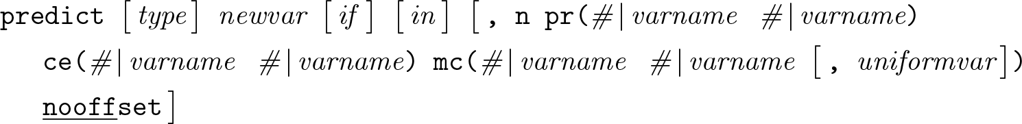
Description

Following intcount, the predict command can be used to construct several measures conditional on covariate values, including the expected count, the probability of the count falling in a specified interval, and the expected value of the count, conditional on it lying in a specified interval. One can also generate a random draw of the intervalspecific conditional count distribution. These predict options are particularly useful for interpolation purposes. The specified type of prediction is returned in newvar as a double precision variable.

Options

n, the default, gives a prediction of the count conditional only on the covariates.

pr(# | varname # | varname) is the predicted probability (conditional on covariate val-

ues) that the count lies in the interval defined by lower and upper limits that may each be a fixed number or a variable.

ce(# | varname # | varname) is the expectation of the count conditional on the covariates and the event that it lies in the interval defined by the two limits that may be variable or constant.

mc(# | varname # | varname [ , uniformvar ] ) generates a single random draw from the distribution of y conditional on the event that it lies in the interval defined by the two specified limits. If the uniformvar option is not used, intcount will generate the required pseudo–random numbers itself without resetting the random-number seed. Optionally, the simulation can be controlled completely by passing a variable containing uniform pseudo–random numbers. The mc() option is useful for Monte Carlo simulation or imputation applications where distributional characteristics beyond the conditional mean are required.

nooffset causes offset or exposure adjustments to be ignored. By default, any offset or exposure adjustment used for estimation will also be incorporated in the predictions of type pr(), ce(), or n.

4 An application to healthcare demand

We apply the intcount command to data from wave 7 of the Understanding Society UK panel on the use of healthcare services. The questions distinguish three services: consultations with a general practitioner (GP), attendance at a hospital outpatient (OP) clinic, and hospital inpatient (IP) stays.⁴ The first two dependent variables come from the following survey questions:

“In the last 12 months, approximately how many times have you talked to, or visited a GP or family doctor about your own health? Please do not include any visits to a hospital.”

“And in the last 12 months, approximately how many times have you attended a hospital or clinic as an out-patient or day patient?”

Responses to these questions are reported as one of five intervals: 0, [1–2], [3–5], [6–10], 11 or more. Figure 1 shows the two empirical distributions.

Figure 1.

Distributions of the number of GP and OP consultations in the preceding 12 months (UK Household Longitudinal Study [UKHLS wave 7; n = 6822])

The third question is

“In the last 12 months, in all, how many days have you spent in a hospital or clinic as an in-patient?” Answers are given as “exact” integers.

The distribution of responses, shown in the first panel of figure 2 (here plotted over 0–10 days), is typical of count data for rare events. There is a large mode at zero and a highly skewed and dispersed distribution of positive values—the sample maximum is 182 days in this case. This distribution can pose challenging modeling and computational problems. The second panel of figure 2 shows the distribution after we artificially group the responses to conform with the reporting intervals used in the GP and OP questions. Note that ex post grouping should not be assumed to coincide automatically with the answer that would have been provided by the respondent given an interval response scale—respondent behavior may be influenced by question design.

Figure 2.

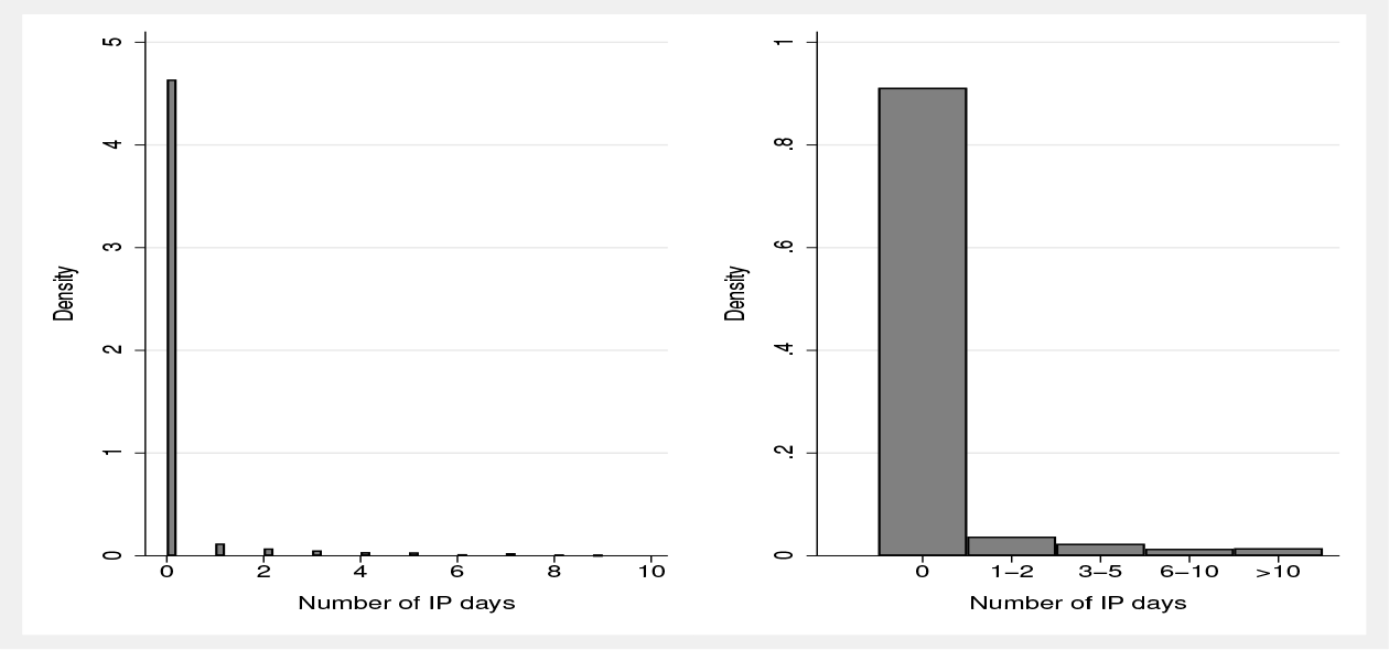
Distribution of the number of days as a hospital inpatient in the preceding 12 months, as observed and after grouping (UKHLS wave 7; n = 6824)

4.1 Hospital IP days: The effect of grouping

First, consider the choice of distributional form, using the original exact data. The intcount command can accommodate exact count data by setting the upper and lower limit variables equal to the exact count. The resulting estimates reproduce exactly those produced by poisson or zip for the Poisson model, binreg for the binomial model,⁵ and nbreg or zinb for the negative binomial model. The covariates used in these models are simple demographics: a cubic in age a (measured in decades from an origin of 50 years), membership of any ethnic minority nonw, an indicator for the absence of any educational qualification noed, and another for degree-level education degree. The following code produced alternative gender-specific models, whose sample fit is summarized in table 1 using the Akaike information criterion (AIC) and Bayesian information criterion (BIC).

Table 1.

AIC and BIC for zero-inflated versions of Poisson, binomial, and negative binomial count-data models, estimated separately by gender from exact data on days spent in hospital

Distributional form		Women				Men
		AIC		BIC		AIC	BIC
Without zero inflation
Poisson	91295		91350		71859		71913
Binomial	93874		93929		73634		73687
Negative binomial	21536		21599		13586		13647
With zero inflation
Poisson	43165		43274		30237		30343
Binomial	45494		45604		31743		31850
Negative binomial	21456		21573		13443		13557

It is clear from table 1 that the negative binomial model is far superior in terms of sample fit to the Poisson and binomial models and also that zero inflation improves the fit substantially.

We now investigate the effect of data grouping by refitting the model using the artificially grouped form of the variable whose distribution is shown in figure 2. The code is as follows:

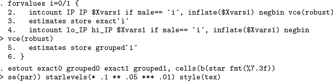
Table 2 compares the parameter estimates. There are substantial parameter differences, particularly for the age and education effects in the female sample.

Table 2.

Estimates of zero-inflated negative binomial model fit from exact and artificially grouped data

Parameter (std. err.)		Women				Men
Parameter (std. err.)		Exact		Grouped		Exact		Grouped
Base model parameters
age^§	0.042		0.102*		0.078		0.177**
age^§	(0.117)		(0.061)		(0.096)		(0.076)
age²	0.057**		0.030**		0.024		0.006
age²	(0.027)		(0.015)		(0.028)		(0.020)
age³	−0.001		0.006		0.005		0.001
age³	(0.014)		(0.008)		(0.011)		(0.008)
Nonwhite	0.155		0.067		−0.350		−0.260
Nonwhite	(0.192)		(0.101)		(0.232)		(0.180)
No education	0.092		0.027		0.203		0.114
No education	(0.173)		(0.112)		(0.209)		(0.173)
Degree	0.018		−0.229**		−0.753***		−0.660***
Degree	(0.204)		(0.107)		(0.223)		(0.171)
Intercept	−0.426**		0.769***		0.713**		1.219***
Intercept	(0.206)		(0.186)		(0.299)		(0.273)
lnalpha	3.072***		1.267***		2.856***		1.601***
lnalpha	(0.114)		(0.276)		(0.146)		(0.355)
age^§	0.899***		0.258***		−0.320***		−0.216***
age^§	(0.169)		(0.054)		(0.094)		(0.051)
age²	−0.539		−0.022**		−0.094***		−0.041***
age²	(0.627)		(0.010)		(0.031)		(0.013)
age³	−0.263		−0.027***		−0.016		−0.003
age³	(0.170)		(0.007)		(0.010)		(0.006)
Nonwhite	−0.056		−0.052		−0.120		−0.015
Nonwhite	(0.276)		(0.079)		(0.166)		(0.110)
No education	−0.710*		−0.202**		−0.132		−0.106
No education	(0.393)		(0.086)		(0.171)		(0.107)
Degree	0.337		−0.011		0.034		0.051
Degree	(0.279)		(0.081)		(0.178)		(0.114)
Intercept	−0.341		1.494***		0.695***		1.735***
Intercept	(0.377)		(0.214)		(0.248)		(0.272)

NOTES: § Age measured in decades from an origin of 50. Statistical significance: * = 10%, ** = 5%, *** = 1%

Figure 3 shows the implications of parameter differences for the estimated age profiles, plotting the probability of hospitalization Pr(y > 0|age) against age in the range 16–85, with other covariates set to modal zero values. The relevant code is as follows:

Figure 3.

Predicted age profile of zero-count probability by age for ethnic majority woman and man with midlevel education

The estimated age profiles remain broadly similar after grouping, but they display more variability for the estimates based on exact data, so coarsening the counts to interval form has a smoothing effect in this example.

It is also striking in this application that grouping has a perverse effect on the standard errors. It is clear theoretically that recoding count data to coarser interval form must reduce statistical precision of the parameter estimator for a well-specified count-data model (this is easily confirmed empirically using Monte Carlo simulation by applying intcount to simulated counts in exact and grouped form). However, the anticipated loss of precision may not occur for computed standard errors when the count-data model is misspecified. A poor model may do well in fitting the distribution of responses within broad intervals but much worse in fitting the distribution of exact counts within those intervals. Parameter estimates may be (asymptotically) biased differently for grouped and exact data, and the computed confidence intervals (that are not statistically valid for misspecified models) need not be wider for the interval estimates. This is what we find in table 2, where the interval estimates have robust standard errors that are almost always smaller (and in many cases much smaller).

4.2 Interpolated healthcare measures

The intcount command has been designed to be used for interpolation of the underlying count from coarse interval data. We now turn attention to the GP and OP variables, again taking the negative binomial as our basic model but considering both standard and zero-inflated (probit) variants. As covariates, we use dummy variables to allow for gender and ethnicity effects, a cubic in age, and a four-level categorization of educational attainment. Table 3 gives results and also includes estimates of the logit variant for the OP data. Comparison of the fourth and fifth columns of table 3 confirms that the choice between probit and logit specifications makes virtually no difference to the estimates except for scaling of the zero-inflation coefficients (which are larger in absolute value for the logit model by approximately $\sqrt{π^{2} / 3} = 1.814$ ).

Table 3.

Estimates of negative binomial models for counts of GP and hospital OP consultations, estimated from grouped data

Parameter (std. err.)		GP consultations		Hospital OP consultations
Parameter (std. err.)		No zero inflation	Probit inflation	No zero inflation	Probit inflation		Logit inflation
Base model parameters
age^§		0.094***	0.068***	0.168***	0.065***		0.064***
age^§		(0.009)	(0.009)	(0.014)	(0.016)		(0.016)
age²		0.001	0.001	0.006*	0.003		0.003
age²		(0.002)	(0.002)	(0.003)	(0.004)		(0.004)
age³		0.001	0.002**	0.001	0.006***		0.007***
age³		(0.001)	(0.001)	(0.002)	(0.002)		(0.002)
Male		−0.368***	−0.280***	−0.321***	−0.137***		−0.139***
Male		(0.015)	(0.016)	(0.023)	(0.027)		(0.027)
Minority		−0.139***	−0.130***	0.046*	0.012		0.016
Minority		(0.017)	(0.018)	(0.027)	(0.031)		(0.031)
GCSE		−0.148***	−0.147***	−0.052	−0.085**		−0.084**
GCSE		(0.021)	(0.021)	(0.033)	(0.035)		(0.035)
A-level		−0.268***	−0.271***	−0.183***	−0.159***		−0.158***
A-level		(0.024)	(0.025)	(0.039)	(0.042)		(0.042)
Degree		−0.350***	−0.373***	−0.158***	−0.203***		−0.201***
Degree		(0.020)	(0.021)	(0.032)	(0.035)		(0.034)
Intercept		1.525***	1.512***	0.616***	0.704***		0.702***
Intercept		(0.022)	(0.022)	(0.036)	(0.040)		(0.040)
ln(α)		0.153***	0.085***	1.146***	0.973***		0.973***
ln(α)		(0.012)	(0.014)	(0.013)	(0.021)		(0.021)
Zero-inflation parameters
age^§	−0.621***			−0.731***		−1.424***
age^§	(0.108)			(0.130)		(0.261)
age²	−0.220**			−0.350***		−0.694***
age²	(0.086)			(0.096)		(0.182)
age³	−0.024			−0.051**		−0.102***
age³	(0.021)			(0.021)		(0.038)
Male	4.645			0.730***		1.291***
Male	(79.355)			(0.080)		(0.154)
Minority	0.163*			−0.107		−0.161
Minority	(0.096)			(0.067)		(0.114)
GCSE	−0.045			−0.218**		−0.367**
GCSE	(0.106)			(0.091)		(0.156)
A-level	−0.131			−0.005		0.008
A-level	(0.128)			(0.095)		(0.161)
Degree	−0.421***			−0.254***		−0.435***
Degree	(0.133)			(0.091)		(0.154)
Intercept	−6.221			−1.397***		−2.470***
Intercept	(79.355)			(0.131)		(0.256)
AIC		94783	94639	75310	75054		75055
BIC		94867	94799	75394	75214		75215

NOTES: § Age measured in decades from an origin of 50. Statistical significance: * = 10%, ** = 5%, *** = 1%

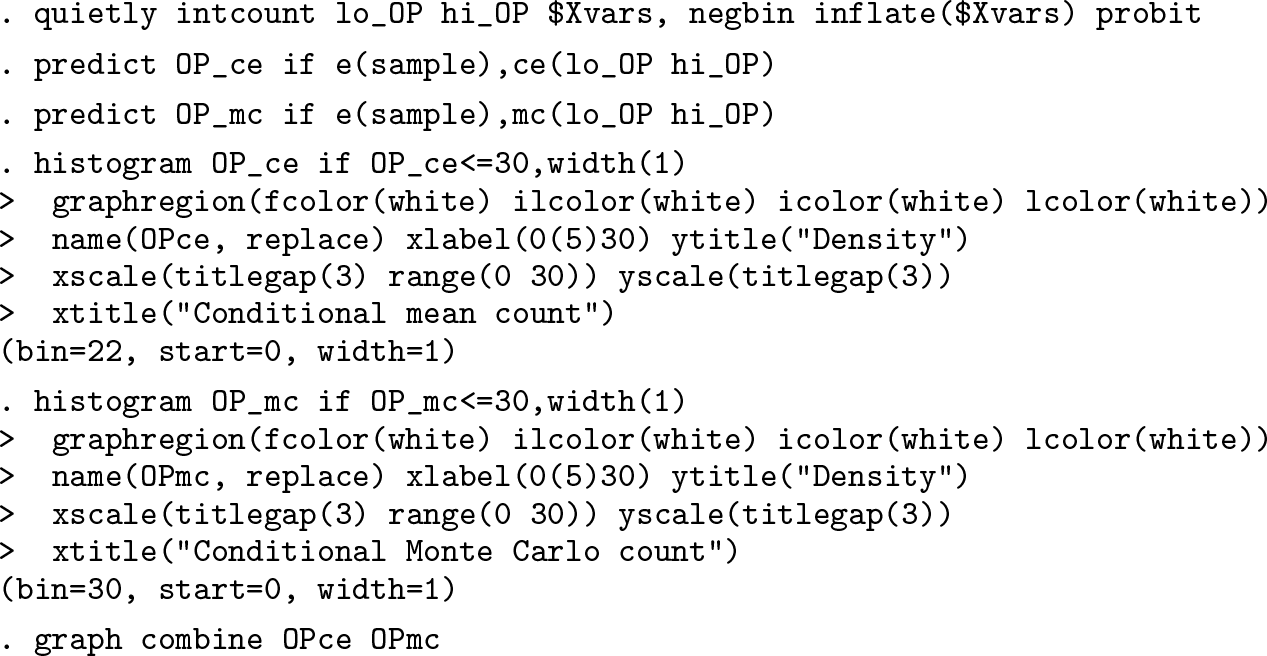
We now compare two interpolation methods. If the observed interval is [L_i, U_i], the conditional expectation predictor of the unobserved true count is E(y| X _i, L_i, U_i), and this is specified by the ce() option of the predict command.⁶ The alternative is to generate a random draw from the conditional distribution f(y| X _i, L_i, U_i) using the mc() option. The following code generates the interpolations and plots their distributions (for the example of the OP count):

The distributions for the interpolated GP and OP counts are shown in figures 4 and 5; the ce() interpolator gives a much lumpier distribution than the mc() interpolator because it averages out random variation within intervals.

Figure 4.

Distributions of GP consultation count with conditional expectation and Monte Carlo interpolation

Figure 5.

Distributions of OP consultation count with conditional expectation and Monte Carlo interpolation

Use of the ce() interpolator understates variance, so if other distributional features besides the conditional mean are of interest, the mc() interpolator is usually preferable. The following code produces the means and standard deviations shown in table 4. Within education or gender groups, the mean counts produced by ce() and mc() are similar (they would be essentially identical if we average many mc() interpolations or if there were a large sample within each education group). In contrast, cell-specific sample dispersion clearly confirms the downward bias in variance for the ce() interpolator.

Table 4.

Means and standard deviations of GP and hospital OP consultations interpolated by alternative methods

Education level		Women				Men
Education level		ce()		mc()		ce()		mc()
GP consultations
None	4.28		4.31		3.36		3.34
None	[4.98]		[5.53]		[4.25]		[4.39]
GCSE 3.38	3.41		2.41		2.42
GCSE 3.38	[4.13]		[4.51]		[3.42]		[3.59]
A-level	3.06		3.08		1.90		1.91
A-level	[3.64]		[3.88]		[2.77]		[2.96]
Degree	2.80		2.82		1.99		2.01
Degree	[3.44]		[3.65]		[2.73]		[2.88]
OP consultations
None	2.04		2.00		1.91		1.86
None	[3.79]		[3.94]		[3.67]		[3.83]
GCSE	1.70		1.63		1.36		1.27
GCSE	[3.31]		[3.22]		[2.91]		[2.91]
A-level	1.54		1.49		1.03		0.94
A-level	[3.07]		[3.08]		[2.42]		[2.34]
Degree	1.56		1.51		1.16		1.07
Degree	[2.99]		[2.95]		[2.55]		[2.45]

NOTES: Group-specific standard deviations in square brackets.

4.3 Determinants of future healthcare demand

The UKHLS is a perpetual panel, and, in addition to healthcare use in wave 7, we can also observe a range of health measures and other characteristics at the wave 2 baseline. We use this rather than wave 1 as the baseline because a range of objective measurements was made by nurse interviewers at wave 2.

Our analysis dataset covers demographic covariates (age, gender); indicators of socioeconomic status (homeownership, log equivalized household income, education); and biometrics (waist–height ratio, grip strength, resting heart rate, lung function, HDL “good” cholesterol, hypertension). We fit standard negative binomial models from the interval data on GP and OP consultations. The following code produces three variants of the model for each dependent variable, and the parameter estimates are shown in table 5:

Table 5.

5-year-ahead predictive models of healthcare use

	GP consultations			OP consultations
Coefficient	(1)	(2)	(3)	(1)	(2)	(3)
Male	−0.287***	−0.170**	−0.176**	−0.278***	−0.197*	−0.194
Male	(0.044)	(0.075)	(0.075)	(0.072)	(0.119)	(0.119)
Age^§	0.090***	0.032*	0.035*	0.166***	0.144***	0.146***
Age^§	(0.015)	(0.018)	(0.019)	(0.025)	(0.030)	(0.032)
Age squared§	0.022***	0.026***	0.022**	0.034**	0.036**	0.036**
Age squared§	(0.008)	(0.008)	(0.009)	(0.014)	(0.014)	(0.015)
Homeowner	−0.138**		−0.095	−0.071		−0.023
Homeowner	(0.062)		(0.062)	(0.101)		(0.103)
ln(income)	−0.103**		−0.051	0.083		0.117*
ln(income)	(0.041)		(0.042)	(0.068)		(0.069)
No qualification	0.122		0.097	0.069		0.065
No qualification	(0.080)		(0.080)	(0.134)		(0.133)
Degree	−0.015		0.006	−0.114		−0.113
Degree	(0.047)		(0.047)	(0.077)		(0.077)
Waist–height ratio		0.143***	0.132***		0.111**	0.114**
Waist–height ratio		(0.027)	(0.027)		(0.045)	(0.045)
Grip strength		−0.117***	−0.109***		−0.100*	−0.111**
Grip strength		(0.036)	(0.036)		(0.055)	(0.055)
Pulse rate		−0.010	−0.012		0.028	0.028
Pulse rate		(0.022)	(0.022)		(0.036)	(0.037)
Lung function		−0.039	−0.032		0.034	0.039
Lung function		(0.037)	(0.037)		(0.060)	(0.061)
HDL cholesterol		−0.060**	−0.060**		0.016	0.010
HDL cholesterol		(0.025)	(0.025)		(0.041)	(0.041)
Hypertension		0.096*	0.096*		−0.054	−0.057
Hypertension		(0.053)	(0.053)		(0.088)	(0.088)
Intercept	1.714***	0.745***	1.205***	−0.241	0.241***	−0.560
Intercept	(0.298)	(0.042)	(0.304)	(0.491)	(0.068)	(0.503)
ln(α)	−0.053	−0.084*	−0.087**	1.073***	1.068***	1.065***
ln(α)	(0.043)	(0.043)	(0.043)	(0.044)	(0.044)	(0.044)
AIC	8866	8811	8811	7279	7276	7280
BIC	8921	8878	8903	7334	7343	7371

NOTES: ^§ Age measured in decades from an origin of 50. Statistical significance: * = 10%, ** = 5%, *** = 1%

There is little evidence of a predictive role for socioeconomic status variables when the biometrics are included in the model, so we adopt variant (2), which uses only demographic and biometric covariates. Among the biometrics, only waist–height ratio and grip strength have a consistently significant impact, and the following code uses the n predict option to quantify those impacts by computing the mean predicted effect of adding 1 standard deviation to each in turn. The effects are substantial in terms of the potential cost to the public healthcare system: a uniform 1 standard deviation increase in waist–height ratio increases the consultation workload by 15% for GPs and 12% for hospital OP clinics. A similar increase in the grip strength measure is predicted to produce an 11% reduction in GP workloads and a 10% reduction for OP clinics.

5 Conclusions

Survey count data often come in interval form rather than exact counts. It is common for ad hoc methods to be used for modeling such data—for example, regression applied to midpoint interpolations, or ordered probit regression that does not exploit the known interval limits or the count nature of the data. In this article, I presented a new command, intcount, which allows the estimation of a range of count-data regression models from interval data without making arbitrary approximations. The postestimation predict command allows the use of the fitted model for many prediction purposes, including interpolation of the unobserved underlying exact count.

I illustrated the use of intcount with applications to data from the UK Understanding Society panel on the health service use. These applications demonstrate that interval observation need not be a barrier to econometric analysis.

7 Programs and supplemental materials

Supplemental Material, st0571 - intcount: A command for fitting count-data models from interval data

Supplemental Material, st0571 for intcount: A command for fitting count-data models from interval data by Stephen Pudney in The Stata Journal

Footnotes

6 Acknowledgments

I am grateful to Apostolos Davillas for help with preparing data from Understanding Society, which is an initiative funded by the Economic and Social Research Council and various government departments, with scientific leadership by the Institute for Social and Economic Research, University of Essex, and survey delivery by NatCen Social Research and Kantar Public. The research data are distributed by the UK Data Service. This work was supported by the Economic and Social Research Council through the project How can biomarkers and genetics improve our understanding of society and health? (grant ES/M008592/1), the Centre for Micro-Social Change (grant ES/L009153/1), and the Understanding Society study (grant ES/K005146/1). I am extremely grateful to the editors and an anonymous reviewer for comments that have greatly improved the code and its presentation in this article. The views expressed in this article, and any errors or omissions, are mine alone.

7 Programs and supplemental materials

To install a snapshot of the corresponding software files as they existed at the time of publication of this article, type

Notes

References

Cameron

A. C.

Trivedi

P. K.

. 2013. Regression Analysis of Count Data. 2nd ed. Cambridge: Cambridge University Press.

Davillas

Pudney

. 2019. Baseline health and public healthcare costs five years on: A predictive analysis using biomarker data in a prospective household panel. Understanding Society Working Paper No. 2019-01, Economic & Social Research Council. https://www.iser.essex.ac.uk/research/publications/working-papers/iser/2019-01.pdf.

Manski

Tamer

F.E.

. 2002. Inference on regressions with interval data on a regressor or outcome. Econometrica 70: 519–546.

StataCorp. 2017. Stata 15 Mata Reference Manual. College Station, TX.

Supplementary Material

Please find the following supplemental material available below.

For Open Access articles published under a Creative Commons License, all supplemental material carries the same license as the article it is associated with.

For non-Open Access articles published, all supplemental material carries a non-exclusive license, and permission requests for re-use of supplemental material or any part of supplemental material shall be sent directly to the copyright owner as specified in the copyright notice associated with the article.

0.18 MB

0.00 MB