
Abstract
A recurring problem in statistics is estimating and visualizing nonlinear dependency between an effect and an effect modifier. One approach to handle this is polynomial regressions of some order. However, polynomials are known for fitting well only in limited ranges. In this article, I present a simple approach for estimating the effect as a contrast at selected values of the effect modifier. I implement this approach using the flexible restricted cubic splines for the point estimation in a new simple command,
Keywords
1 Introduction
A classical approach on effect modifiers is to regress the outcome (all-cause mortality,
In this article, I present an approach where the measure of association between smoking and mortality is split into two log odds-functions dependent on the mean arterial pressure—one for nonsmokers and one for smokers. Contrasting these two log odds-functions gives an estimate of the log odds-ratio at selected values of the effect modifier (mean arterial pressure). Exponentiated, the log odds-ratios give the estimates of the odds ratios. Restricted cubic splines are a simple, flexible way of estimating the possibly nonlinear functions for the unexposed (nonsmokers) and the exposed (smokers) groups. I introduce a simple command,
This article proceeds as follows. Section 2 derives and explains the contrast function in the linear and general cases. Section 3 introduces restricted cubic splines. Section 4 presents the example dataset. Section 5 describes commands in Stata for restricted cubic splines. Section 6 presents a new prefix command,
2 The contrast function
The expected all-cause mortality (

In a logit regression, the expected all-cause mortality is the log odds-function of the mean artery pressure handled independently for nonsmokers and smokers. The contrast function, estimating the log odds-ratio of the effect modifier (

One simple, flexible way to approximate nonlinear functions like f 0(m) and f 1(m) from data points is to use restricted cubic splines.
3 Restricted cubic splines
Cubic splines are functional approximations based on piecewise cubic polynomials (see Harrell [2015], Buis [2009], and Croxford [2016], Orsini and Greenland [2011]).
When a function is possibly nonlinear and unknown except for some data points, cubic splines are a flexible way to approximate the unknown function. Cubic splines are a set of transformations on the independent variable, which together linearly approximate the unknown function. This makes cubic splines useful for nonlinear regression modeling.
A single polynomial

will usually fit observed pairs of X and Y values poorly at some parts of the curve. In splines, X values (ki
)in
=1-named knots are chosen. The combined polynomial spline is the overall cubic polynomial added cubic effects starting at each knot bi
+3 ×max(0, X −ki
)3. By design, the cubic spline has continuous second-order derivatives. Also by design, it is easy to generate variables dependent only on X and the knots, (ki
)in
=1, such that the coefficients,

There is typically a problem with cubic splines at the tails of the curve. It is unknown how the curve should behave when extrapolating the curve beyond the range of X.
To avoid inheriting false curvature from the center of the curve, one can restrict the splines to be linear beyond the range of the knots, hence restricted cubic splines.
To achieve linearity at the left side of the range of X for a restricted cubic spline, one removes the quadratic
There are guidelines (Harrell 2015, 26) covering most datasets for choosing the knots and their numbers. In summary, they are the following:
use fixed percentiles for the marginal distribution of the effect modifier to ensure enough points in each interval and guarding against outliers overly influencing knot placement; choose a number of knots between 3 (small datasets, number of observations around 100) and 7; if the number of observations is less than 100, choose the fifth-smallest and the fifth-largest observation as outer knots; choosing more than five knots is seldom necessary; often, choosing four knots is a good choice; and Akaike’s information criterion (AIC) can be used for data-driven comparisons of the number of knots and where to place them.
4 The example data
The example dataset is the Whitehall 1 dataset, which consists of data on 18,403 male British Civil Servants employed in London (StataCorp 2017; Royston and Sauerbrei 2008):
. use all10 cigs map using http://www.stata-press.com/data/r15/smoking.dta (Smoking and mortality data)
The outcome is 10 years all-cause mortality (variable
The exposure variable . generate smoker = (cigs > 0) if !missing(cigs) . label variable smoker "Smoking at baseline" . label define smoker 0 "No" 1 "Yes" . label values smoker smoker
The effect modifier is
5 Restricted cubic splines in Stata
In Stata, to generate a set of restricted cubic spline variables for regressions, use the command
The package
Orsini and Greenland (2011) extend the package
The goal for both Buis (2008) and Orsini and Greenland (2011) is to model the dependency between the outcome and a continuous exposure. The first uses restricted cubic splines, while the latter is more flexible.
My approach in this article is to estimate a measure of association (a contrast or a function of one) as a function of a selected set of values of an effect modifier by estimating each part of the contrast as a function separately and then estimating the contrast by the difference between the two functions for each of the selected values.
Using four knots, we can estimate the contrast function (from section 2) of the coefficients by the following four steps for the example dataset:
Estimate restricted cubic splines for nonsmokers. Spline values are missing for smokers:
. mkspline _map0 = map if !smoker & !missing(smoker, map), cubic nknots(4) Estimate restricted cubic splines for smokers. Spline values are missing for non-smokers:
. mkspline _map1 = map if smoker & !missing(smoker, map), cubic nknots(4) Set missing values for the splines to be zero. This way, the estimates on splines for nonsmokers are independent of the estimates on splines for smokers:
. mvencode _map??, mv(0) override (output omitted) Do the logit regression:

The variables
To predict the contrasts at selected values of the effect modifier is more complex.
The independent variables from restricted cubic splines are transformations of the effect modifier, and these transformations cannot be handled by, for example,
To use
6 The emc command
6.1 Syntax
. emc, at(numlist)
6.2 Options
twoway_options change the default graph.
6.3 Description
The prefix command
For each value in numlist specified in the
The calculations in difference in means using odds ratios using odds ratios in a matched study using risk differences using relative risks using hazard ratios using incidence-rate ratios using
One can also analyze contrasts in
I developed
6.4 Stored results

7 Comparing emc prefix command with other approaches
This section compares an application of the

Four approaches (linear, quadratic, stratified, and
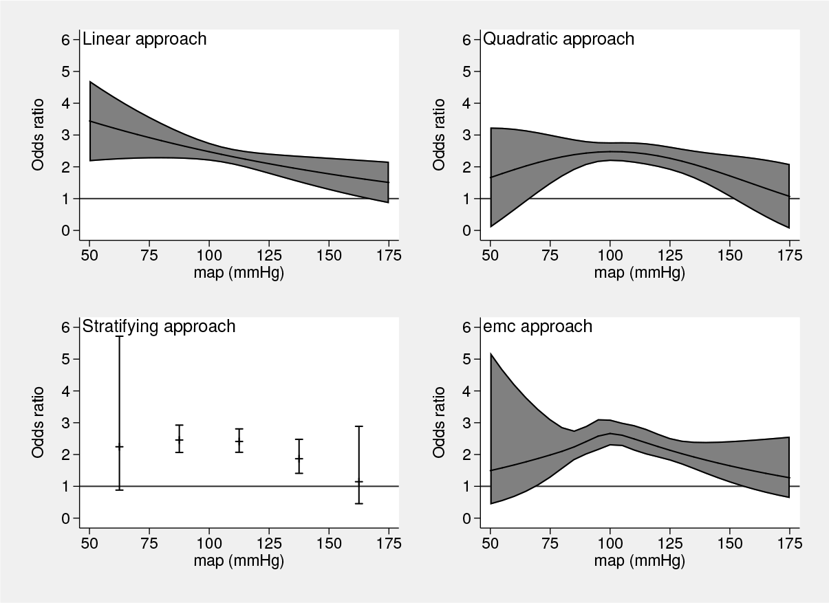
Four approaches (linear, quadratic, stratified, and
The first approach reported in figures 1 and 2 is linear. Here the log odds are modeled in a logit model with the main effects of
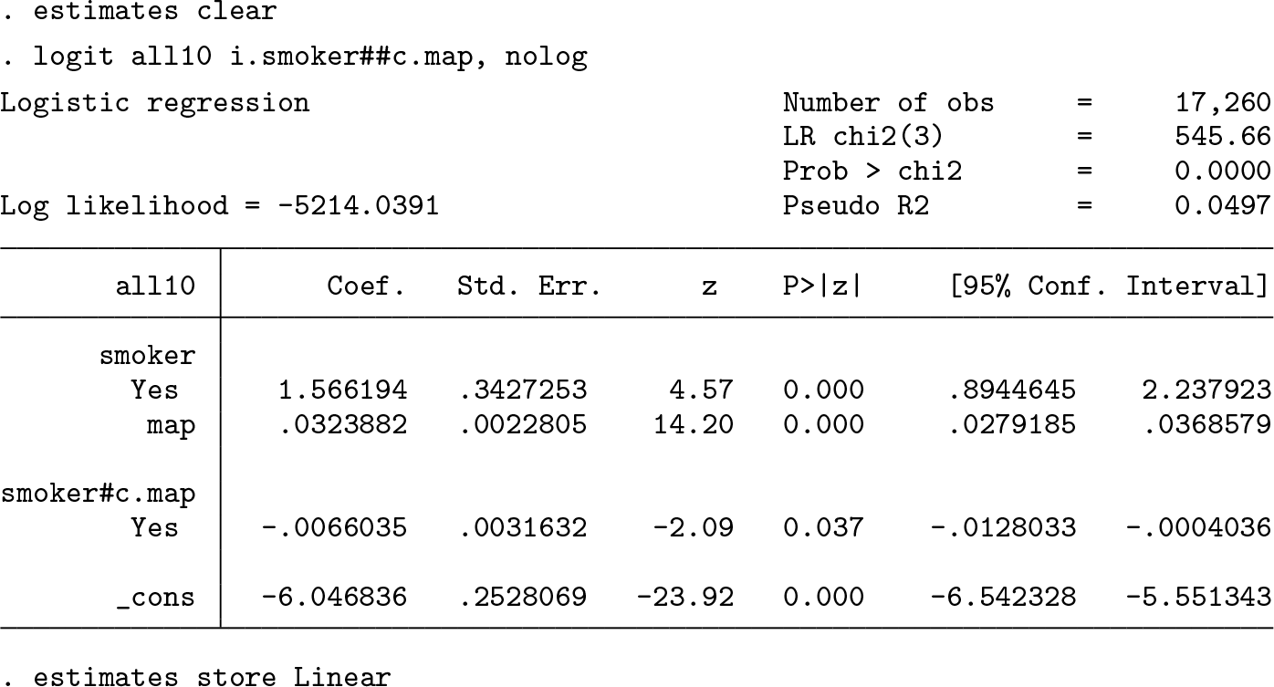
First, we estimate the log odds-ratios using . margins, at(map=(50(5)175)) expression(_b[1.smoker]+_b[1.smoker#map]*map) (output omitted)
We save estimates and confidence intervals in matrices for graphing:
. matrix tmp = r(at), r(table)´ . matrix Linear = tmp[1…,"map"], tmp[1…,"b"], tmp[1…,"ll"], tmp[1…,"ul"] (output omitted)
Second, we estimate the odds ratios
. margins, at(map=(50(5)175)) expression(exp(_b[1.smoker]+_b[1.smoker#map]*map)) (output omitted)
We save estimates and confidence intervals in matrices for graphing:
. matrix tmp = r(at), r(table)´ . matrix Linear_exp = tmp[1…,"map"], tmp[1…,"b"], tmp[1…,"ll"], > tmp[1…,"ul"]
The second model is quadratic; that is, there is a quadratic term (

Similarly to the linear case, we estimate the log odds-ratios by using . margins, at(map=(50(5)175)) . > expression(_b[1.smoker]+_b[1.smoker#map]*map+_b[1.smoker#map#map]*map*map) . (output omitted) . matrix tmp = r(at), r(table)´ . matrix Quadratic = tmp[1…,"map"], tmp[1…,"b"], tmp[1…,"ll"], > tmp[1…,"ul"]
Likewise, we estimate the odds ratios by using . margins, at(map=(50(5)175)) . > expression(exp(_b[1.smoker]+_b[1.smoker#map]*map+_b[1.smoker#map#map]*map*map)) . (output omitted) . matrix tmp = r(at), r(table)´ . matrix Quadratic_exp = tmp[1…,"map"], tmp[1…,"b"], tmp[1…,"ll"], > tmp[1…,"ul"]
The third approach is stratifying the mean arterial pressure (
We create the stratifying variable ( . egen map_grp = cut(map), at(50(25)175) (9 missing values generated)
We create the interval midpoints and saved them in a matrix named . mata: st_matrix("map", (2::6) :* 25 :+ 12.5) . matrix colnames map = map
The main effects of

We again use . margins r.smoker, over(map_grp) predict(xb) (output omitted) . matrix tmp = r(table)´ . matrix tmp = tmp[1…,"b"], tmp[1…,"ll"], tmp[1…,"ul"]
We save interval midpoints and estimates for graphing:
. matrix Stratifying = map, tmp
A simple way of exponentiation of a matrix in Stata is to use Mata:
. mata: st_matrix("tmp", exp(st_matrix("tmp"))) . matrix colnames tmp = b ll ul
We save the estimated odds ratios for graphing:
. matrix Stratifying_exp = map, tmp
Finally, we use the
. emc, at(50(5)175) eform: logit all10 smoker map, or (output omitted) . estimates store emc
Table 1 compares the underlying logit models (that is, the models for log odds-ratios) using the AIC and Bayesian information criterion (BIC) from stored estimates for the four approaches and the command

For AIC, the
For both AIC and BIC, the stratifying approach is the worst. As noted in Royston and Sauerbrei (2008, 2), stratification or classification leads to problems with overparameterization, loss of efficiency, and defining cutpoints. Further, “…a cutpoint model is an unrealistic way to describe a smooth relationship between a predictor and an outcome variable.”
Looking at figure 1, we see that the linear approach, compared with the other three approaches, is too simple. The linear model in figure 1 gives poor prediction when the mean arterial pressure is low and hence lesser or wrong insight.
Of course, one can model the curve by adding quadratic or higher terms and using, for example,
The
8 Concluding remarks
I presented a simple approach to model and visualize the dependency of a contrast to a continuous variable based on a regression. However, one can also use this approach in more complex applications, for example, to visualize the difference in development between two sets of predicted values, such as the difference in development of unemployment in two countries over time. In this article, I presented a command,
Other techniques than restricted cubic splines, such as fractional polynomials (Royston and Sauerbrei 2008; StataCorp 2017), are alternatives.
10 Programs and supplemental materials
Supplemental Material, st0567 - Visualizing effect modification on contrasts
Supplemental Material, st0567 for Visualizing effect modification on contrasts by Niels Henrik Bruun in The Stata Journal
Footnotes
9 Acknowledgment
I thank Professor Henrik Støvring, Department of Public Health, Aarhus University for help and comments. Thanks also to the reviewer for all his help in the review process.
10 Programs and supplemental materials
To install a snapshot of the corresponding software files as they existed at the time of publication of this article, type
References
Supplementary Material
Please find the following supplemental material available below.
For Open Access articles published under a Creative Commons License, all supplemental material carries the same license as the article it is associated with.
For non-Open Access articles published, all supplemental material carries a non-exclusive license, and permission requests for re-use of supplemental material or any part of supplemental material shall be sent directly to the copyright owner as specified in the copyright notice associated with the article.