Sage Journals: Discover world-class research

Abstract

Statistical methods that quantify the discourse about causal inferences in terms of possible sources of biases are becoming increasingly important to many social-science fields such as public policy, sociology, and education. These methods are also known as “robustness or sensitivity analyses”. A series of recent works (Frank [2000, Sociological Methods and Research 29: 147–194]; Pan and Frank [2003, Journal of Educational and Behavioral Statistics 28: 315– 337]; Frank and Min [2007, Sociological Methodology 37: 349–392]; and Frank et al. [2013, Educational Evaluation and Policy Analysis 35: 437–460]) on robustness analysis extends earlier methods. We implement these recent developments in Stata. In particular, we provide commands to quantify the percent bias necessary to invalidate an inference from a Rubin causal model framework and the robustness of causal inferences in terms of correlations associated with unobserved variables.

Keywords

st0565 konfound mkonfound pkonfound causal inferences bias confounding robustness or sensitivity analyses

1 Introduction

Statistical inferences are often challenged on their uncontrolled bias. There may be bias due to uncontrolled confounding variables or nonrandom selection into a sample. Methods for sensitivity analysis have been developed to assess the robustness of inferences to various sources of bias and inform debate about causal inference. However, most of the previous methods either accounted only for particular sources of bias (such as an unobserved variable) or applied only to certain types of data (such as the categorical treatment variable; see DiPrete and Gangl [2004]; Gill and Robins [2001]; Robins [1987]; Robins, Rotnitzky, and Scharfstein [2000]; Rosenbaum [1986, 2002]; Scharfstein and Irizarry [2003]; VanderWeele [2010]; and VanderWeele and Arah [2011]). In a series of articles (Frank [2000]; Pan and Frank [2003]; Frank and Min [2007]; and Frank et al. [2013]), researchers have extended previous work and developed two robustness-analysis frameworks. The first uses Rubin’s causal model to interpret how much bias there must be to invalidate an inference in terms of replacing observed cases with counterfactual cases or cases from an unsampled population. The second quantifies the robustness of causal inferences in terms of correlations associated with unobserved variables in a regression framework.

In this article, we introduce the konfound command, which implements the two robustness-analysis methods described above in Stata. Specifically, konfound can be used to implement the robustness analysis for the user’s model; the mkonfound command can be used to implement the robustness analysis for multiple studies; and the pkonfound command can be used to implement the robustness analysis for a single published study. Next, we briefly discuss the foundations of these two methods and describe how to use konfound in Stata. For a longer introduction of the methods and more technical details, readers should refer to Frank (2000), Pan and Frank (2003), Frank and Min (2007), and Frank et al. (2008, 2013).

2 Robustness of an inference

2.1 Impact threshold for an omitted confounding variable

In observational studies and quasiexperiments, a key concern pertaining to causal inference is the omitted variable bias problem. That is, there are some unobserved confounding variables that may be correlated with both the outcome and the predictor of interest, which will bias the estimates of the model and thus invalidate inferences. To quantify the impact of a confounding variable necessary to alter a statistical inference, Frank (2000) defined the impact of a confounding variable as r_x _· _cv r_y _· _cv, where r_x _· _cv is the correlation between the unobserved confound and the predictor of interest and r_y _· _cv is the correlation between the unobserved confound and the outcome. For example, if the relationship of interest is between one’s father’s occupation (X) and one’s own educational attainment (Y ), an omitted confounding variable might be one’s father’s education (cv). And the index developed by Frank (2000) allows us to quantify the impact of father’s education in terms of its correlation with the predictor father’s occupation and its correlation with the outcome—educational attainment. Frank (2000) then shows how strongly an omitted confounding variable (cv) would have to be correlated with the predictor (father’s occupation, X) and the outcome (educational attainment, Y ) to invalidate an inference of the effect of X on Y

Figure 1.

The impact of a confounding variable on a regression coefficient

Formally, the calculations follow a partial correlation framework (for more details, see Frank [2000] and Pan and Frank [2004]). For a bivariate regression,

Y = β_{0} + β_{1} X + e

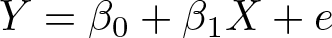
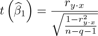
the correlation between X and $Y - r_{y}_{\cdot x}$ can be obtained following

t ({\hat{β}}_{1}) = \frac{r_{y \cdot x}}{\sqrt{\frac{1 - r_{y \cdot x}^{2}}{n - q - 1}}}

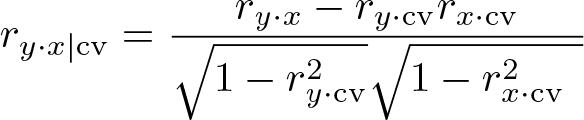
where t is the t ratio of ${\hat{β}}_{1}$ to its standard error from a fit model, n is the sample size, q is the number of parameters estimated (other than the intercept) in the model, and the partial correlation between X and Y after controlling for the confounding variable $cv - r_{y \cdot x}_{| c v}$ can be represented as

r_{y \cdot x | c v} = \frac{r_{y \cdot x} - r_{y \cdot c v} r_{x \cdot c v}}{\sqrt{1 - r_{y \cdot c v}^{2}} \sqrt{1 - r_{x \cdot c v}^{2}}}

To invalidate an inference, we consider the conditions necessary to reduce $r_{x \cdot y | c v}$ below a threshold, $r^{#}$ , for making an inference. Here where t _critical is decided by the significance level (for example, for significance level of 0.05 and a two-sided test with degrees of freedom > 200, t _critical = 1.96).

r^{#} = \frac{t_{critical}}{\sqrt{(n - q - 1) + t^{2}_{critical}}}

To calculate the correlations associated with an omitted confounding variable necessary to invalidate an inference, assume the component correlations are equal, $r_{x}_{\cdot c v} = r_{y}_{\cdot c v}$ , which generates the largest change from $r_{x}_{\cdot y}$ to $r_{x \cdot y | c v}$ for a given product = $r_{x}_{\cdot c v} \times r_{y}_{\cdot c v}$ = impact (Frank 2000). Then, from Frank (2000), impact = $r_{x}_{\cdot c v} \times r_{y}_{\cdot c v} = r_{x}_{\cdot c v} \times r_{x}_{\cdot c v} = r_{y}_{\cdot c v} \times r_{y}_{\cdot c v} .$ Next, set the partial correlation $r_{y \cdot x | c v}$ equal to the threshold $r^{#}$ ,

r_{y \cdot x | c v} = \frac{r_{y \cdot x} - r_{y \cdot c v} r_{x \cdot c v}}{\sqrt{1 - r^{2}_{y \cdot c v} {\sqrt{1 - r^{2}}}_{x \cdot c v}}} = \frac{r_{y \cdot x} - impact}{1 - impact} = r^{#}

and then solve for impact:

\begin{array}{l} impact = \frac{r_{y \cdot x} - r^{#}}{1 - | r^{#} |} \end{array}

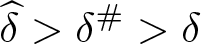
Thus, to invalidate the inference, the impact of the confounding variable $(r_{x}_{\cdot c v} \times r_{y}_{\cdot c v})$ must be greater than

\frac{r_{y} {_{\cdot}}_{x} - r^{#}}{1 - | r^{#} |}

Furthermore, the approach also applies to estimated coefficients that are less than their thresholds, $r^{#}$ . Here is how one alters an inference (assuming r and $r^{#}$ take the same sign):

\begin{array}{l} if : r > r^{#} \Rightarrow impact = \frac{r_{y \cdot x} - r^{#}}{1 - r^{#}} \\ if : r > r^{#} \Rightarrow impact = \frac{r_{y \cdot x} - r^{#}}{1 + r^{#}} \end{array}

Thus, (1) quantifies the smallest impact of the confounding variable necessary to invalidate a statistical inference based on the threshold, r^#.¹

The above calculations can also be extended to models that control for observed covariates as in multiple regression, where the interpretation of the impact and the correlation can be conditioned on other covariates in the model. In the multiple regression case, the raw component correlation before conditioning on covariates can also be derived; interested readers should see Frank (2000). This is available in the konfound command.

2.2 Percent bias necessary to invalidate an inference

A second approach starts by assessing what proportion of an estimate must be due to bias to invalidate an inference (Frank et al. 2013). The proportion is then interpreted in terms of the proportion of observed cases that would have to be replaced with null hypothesis cases to invalidate the inference. These replacement cases can come from counterfactual data as in Rubin’s causal model (Rubin 1974) or from a population from which observed cases were not sampled. This framework enables researchers to identify a “switch point” (Behn and Vaupel 1982) where the bias is large enough to undo one’s belief about an effect (for example, from inferring an effect to inferring no effect). Using the switch point, this framework addresses the concerns pertaining to external validity (such as the extent to which the sampling process has to be biased to invalidate the inference) or concerns pertaining to internal validity (such as the extent to which bias because of uncontrolled preexisting differences can invalidate the inference of the treatment effect).

The approach begins when one compares an estimate with a threshold to represent how much bias there must be to switch the inference. For example, consider figure 2, in which the treatment effect from hypothetical study A (with an estimated effect of 6) and B (with an estimated effect of 8) each exceeds the threshold for making an inference of 4. But note that the estimated effect from study B exceeds the threshold by more than the estimate from study A (assuming that the estimates were obtained with similar levels of control for selection bias in the design of the study and similar levels of precision). Therefore, we state that the inference from study B is more robust than that from study A because a greater proportion of the estimate from study B must be due to bias to invalidate the inference.

Figure 2.

Percent bias necessary to invalidate an inference

To formally derive the percent bias necessary to invalidate an inference, define a population effect as δ, the estimated effect as $\hat{δ}$ , and the threshold for making an inference as $δ^{#}$ . An inference about a positive effect is invalid if That is, an inference is invalid if the estimate is greater than the threshold while the population value is less than the threshold (a symmetric argument applies for negative effects).

\hat{δ} > δ^{#} > δ

To express how much bias there must be in the estimate to invalidate the inference, we can rewrite the above equation as

\hat{δ} - δ > \hat{δ} - δ^{#} > 0

Let’s define bias as bias $(\hat{δ}) = \hat{δ} - δ .$ To invalidate the inference, bias must be larger than the difference between the estimate and the threshold. To express bias as a proportion of the original estimate, we can write

\begin{matrix} bias (\hat{δ}) to invalidate > \hat{δ} - δ^{#} \\ % bias (\hat{δ}) to invalidate = \frac{bias (\hat{δ})}{\hat{δ}} > \frac{\hat{δ} - δ^{#}}{\hat{δ}} = 1 - \frac{δ^{#}}{\hat{δ}} \end{matrix}

For example, in the hypothetical study A in figure 2, percent bias to invalidate the inference = 1 − (4/6) = 1/3. Thus, 33% of the estimate would have to be due to bias to invalidate the inference. In study B, 1 − (4/8) = 50% of the estimate would have to be due to bias to invalidate the inference. Readers should also see Frank et al. (2013) and Frank and Min (2007) for other extensions and more details of the derivations following the Rubin causal model.

3 The konfound command

3.1 Syntax

konfound varlist [, sig( # ) nu( # ) onetail( # ) uncond( # ) rep_0( # )

non_li( # )]

3.2 Description

konfound calculates the impact of an omitted confounding variable necessary to invalidate or sustain an inference for a regression coefficient from the user’s model. It also assesses how strongly an omitted variable has to be correlated with the outcome and the predictor of interest to invalidate or sustain the inference. After fitting a model (such as linear regression), the user can provide a list of variable names, and konfound will produce the impact of an omitted variable (Frank 2000) necessary to invalidate or sustain an inference for each variable. The command will also provide the impact table for all observed covariates in the user’s previous model. These can be used as a benchmark against which to evaluate the impact of an omitted confounding variable necessary to invalidate an inference.

konfound also calculates how much bias there must be in an estimate to invalidate or sustain an inference from the immediately preceding model. After fitting a model (such as a linear regression), users can provide the list of variable names, and konfound will calculate the percent bias needed to invalidate or sustain the inference for each variable in the variable list. The command will also provide sensitivity plots for those variables that are statistically significant in the user’s model.

3.3 Options

sig( # ) specifies the significance level of the test. The default is sig(0.05). To change the significance level to 0.10, use sig(0.1).

nu( # ) specifies the null hypothesis against which to test the estimate. The default is nu(0).

onetail( # ) specifies the one-tail or two-tail test. The default is onetail(0) (two tail). To change to one tail, use onetail(1).

uncond( # ) calculates the impact and component correlations before or after conditioning on covariates in the model. The default is uncond(0), which calculates the impact and component correlations after conditioning on covariates. To change the calculation to before conditioning (unconditional) on covariates, use uncond(1).

rep_0( # ) controls the effect in the replacement cases for percent bias. The default is the null effect (which may or may not be zero). When the null hypothesis is not zero, one can still force the replacement cases to have an effect of zero by assigning rep_0(1).

non_li( # ) specifies the basis for interpreting percent bias to invalidate or sustain an inference for nonlinear models (for example, logit or probit). The default is non_li(0), which uses the original coefficient. To change the calculation based on average marginal effects, use non_li(1).

3.4 Example

To illustrate the use of the konfound command, we use two example datasets from Hamilton (1992). The first example comes from a water use survey reported by Hamilton (1983) from Concord, New Hampshire. The outcome of interest is household water usage in the summer of 1981 (water81). Independent variables include household water usage in the summer of 1980 (water80), household income (income), years of education (educ), whether the head of the household has retired (retire), and number of people in the household in 1980 (peop80).

First, we will regress the outcome on all the independent variables:

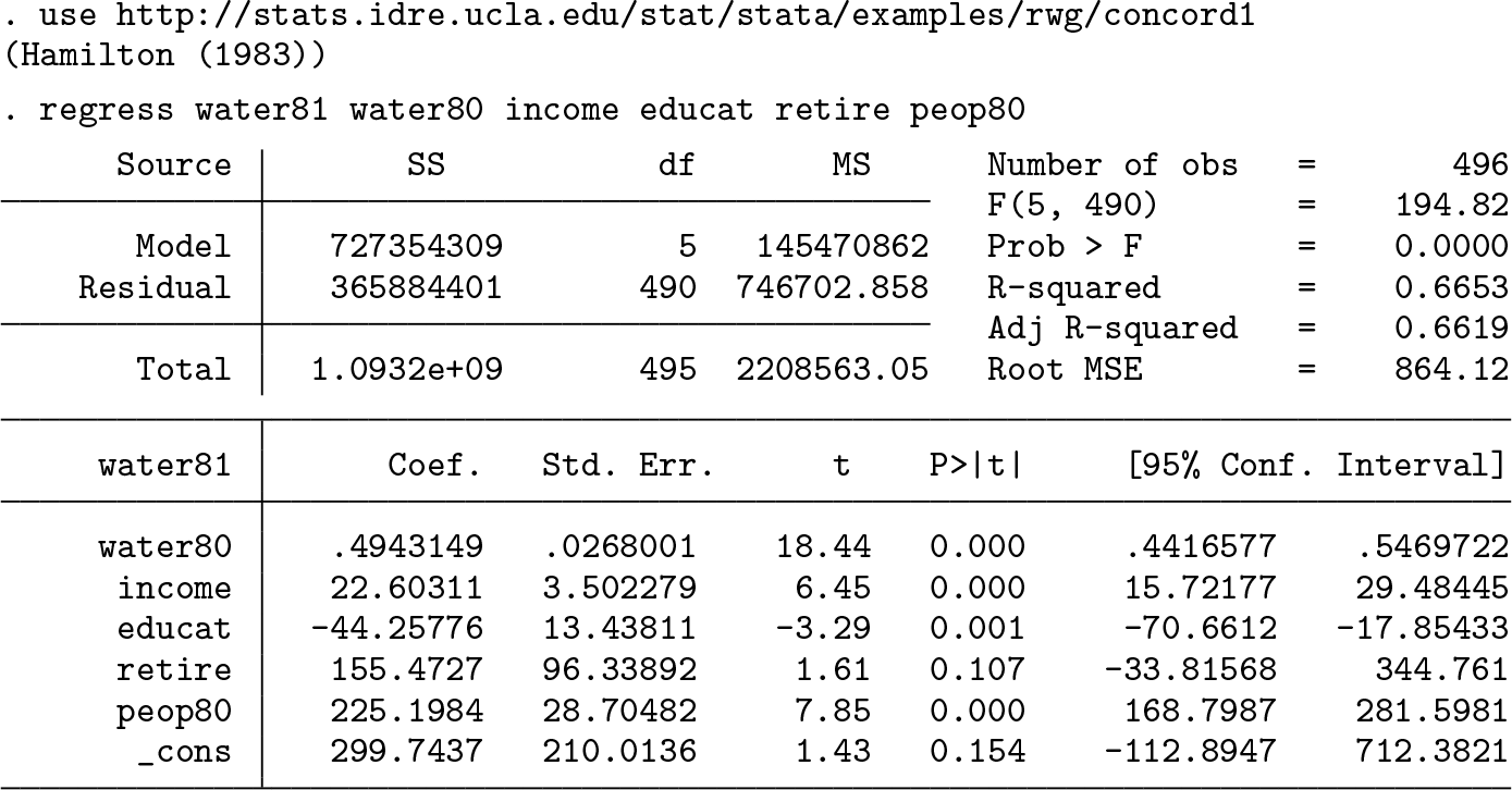
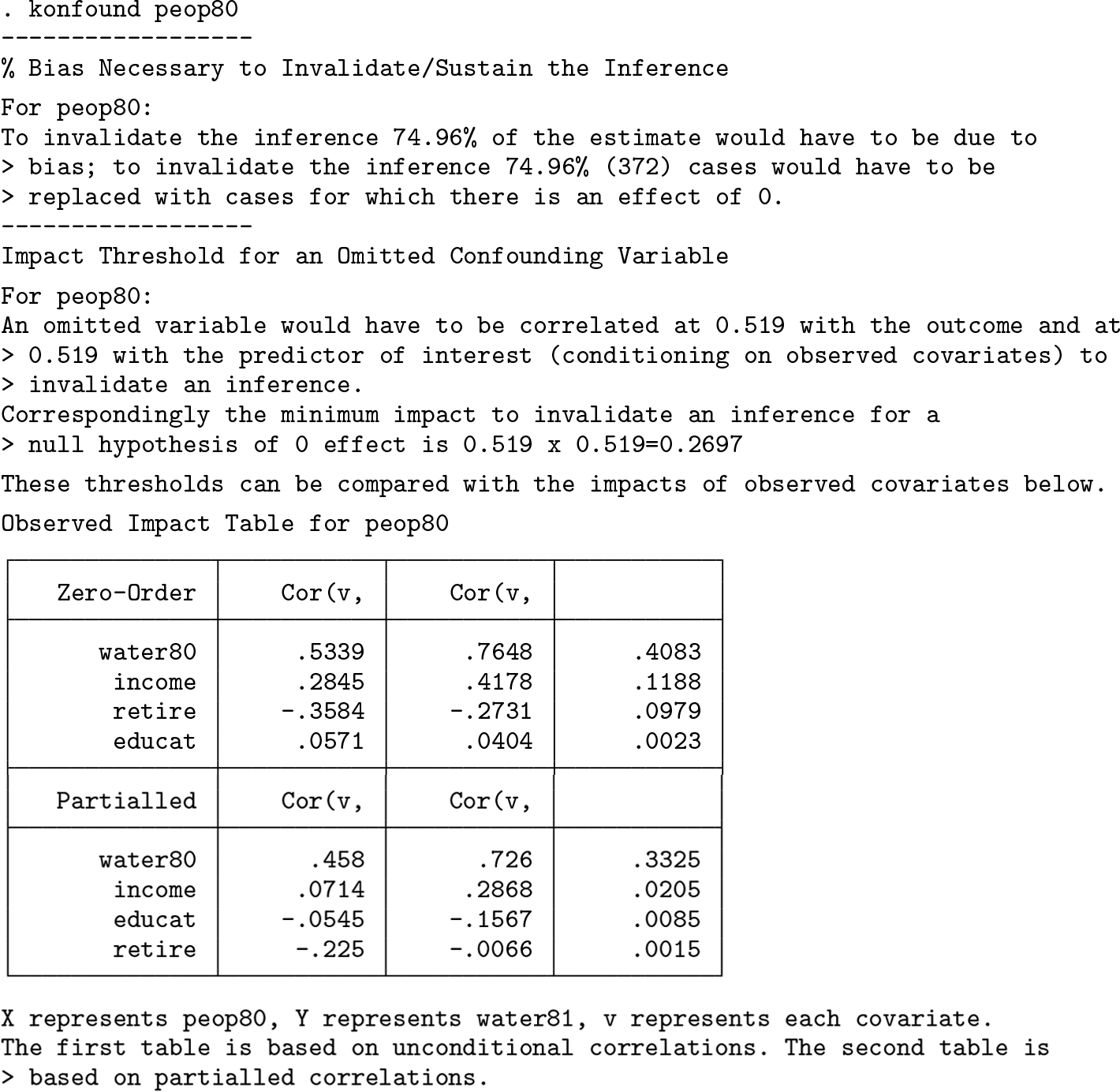
The estimated effect of the number of people in the household (peop80) is statistically significant (p < 0.001). To quantify the robustness of the inference with respect to omitted variables or to quantify the percent of the bias necessary to invalidate the current inference, we use the konfound command:

The first table is based on unconditional correlations. The second table is based on partialled correlations.

The first part of the output calculates the percent bias needed to invalidate the inference for peop80. As it shows, to invalidate the inference, 74.96% of cases (372) would have to be replaced with cases for which there is an effect equal to 0. A graphical illustration is shown in figure 3.

Figure 3.

Percent bias to invalidate the inference for the effect of peop80 on water81

The second part of the output calculates the impact of an omitted variable necessary to invalidate or sustain an inference. First, it shows the impact (0.2697) and the component correlations (0.519) between the omitted variable and the outcome (water81) as well as with the predictor of interest (peop80) that are necessary to invalidate the inference, conditional on other covariates. To calculate impact and component correlation before conditioning on covariates, type

. konfound peop80, uncond(1)

Next, two observed impact tables are shown. For each observed covariate in the model, the first table contains its correlation with the predictor of interest (peop80) and with the outcome (water81) before conditioning on other covariates; similarly, the second table contains the correlation between each covariate and the predictor of interest (peop80) and the outcome (water81) after conditioning on other covariates. These two tables can be used to evaluate the robustness of the inference by comparing the impact of the omitted variable necessary to invalidate the inference with the impact of the observed covariates. For example, figure 4 depicts how the partial correlation between peop80 and water81 would change when we add an omitted confounding variable in the regression. It shows that the impact of an omitted confounding variable necessary to invalidate the inference (ITCV: gray line) would have to be much larger than the impact of income (as well as education and retirement). Furthermore, if the impact of an omitted confounding variable equaled that of prior water usage, the inference would be invalid.²

Figure 4.

Visualization of the impact of an omitted confounding variable on the partial correlation between peop80 and water81

Finally, note several things:

First-time users of konfound need to install three other community-contributed commands—moss, indeplist, and matsort.

Users must run the original regression each time before applying the konfound command.

Bar graphs are generated only for variables that are statistically significant.

Users can evaluate the robustness of inference for multiple variables at the same time; in the previous example, to evaluate the robustness of inference of two variables—peop80 and retire—type

. konfound peop80 retire

The previous example illustrates how the konfound command can be applied to linear regression models.³ The next example illustrates how konfound can be applied to nonlinear models. Note that for a nonlinear model, the impact of an omitted variable necessary to invalidate an inference should not be used, because it is correlation based and thus applies only to linear cases. The percent bias to invalidate the inference can still be applied in this case. However, to calculate the percent bias to invalidate the inference in a nonlinear model, we recommend basing the calculation on the average marginal effect (also known as average partial effect—see Wooldridge [2010]) instead of the original regression coefficient, such that the calculation is robust to different functional forms of the model (for example, logit versus probit).

The next example we use comes from Hamilton (1992), which is from survey data concerning toxic waste in Williamstown, Vermont (Hamilton 1985). The outcome of interest is a dichotomous variable indicating whether the respondent believed the contaminated school should be closed (close). The independent variables include how many years the survey respondent has lived in Williamstown (lived), years of education received (educ), whether the respondent attended more than two health and safety committee meetings (hsc), and whether the respondent is female (female).

First, we run a logistic regression using close as outcome:

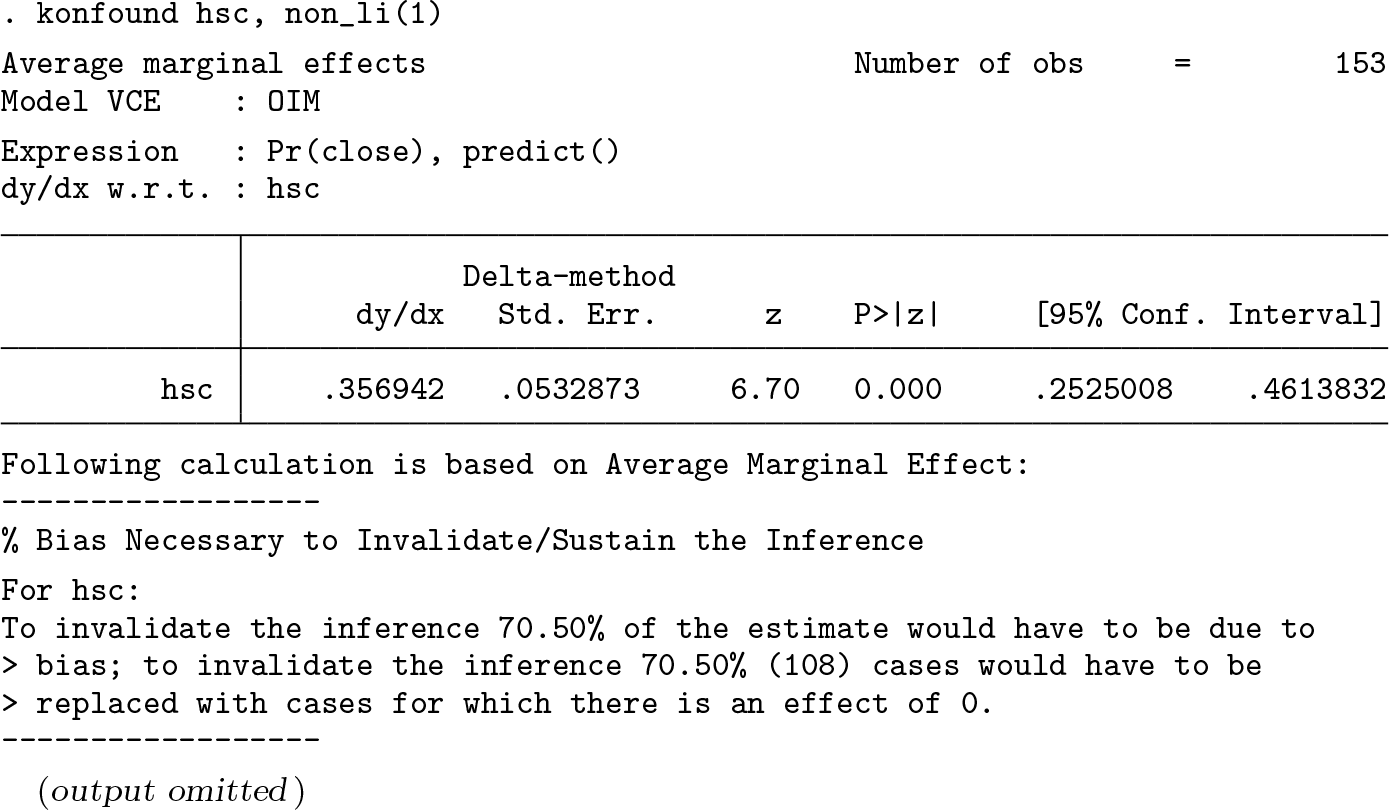
The results show that the estimated effect of hsc is statistically significant (p < 0.001). To calculate the percent bias necessary to invalidate the inference for hsc, we use konfound with a nonlinear model option as below:

Figure 5.

Percent bias necessary to invalidate the inference for the effect of hsc on close

Results show that to invalidate the inference, 70.5% (108) cases would have to be replaced with cases for which there is an effect of 0. The calculation is based on average marginal effects instead of on the original coefficient; in this case, the inference is more robust compared with the calculation based on the original coefficient, which would be 58.23% (89).⁴

4 The mkonfound command

4.1 Syntax

mkonfound var1 var2 [, sig( # ) nu( # ) onetail( # ) rep_0( # ) z_tran( # )]

4.2 Description

mkonfound calculates the impact of an omitted confounding variable necessary to invalidate an inference of a regression coefficient for multiple studies. The command also assesses how strong an omitted confounding variable must be correlated with the outcome and with the predictor of interest to invalidate or sustain the inference for each study. Users input two variables: the observed t ratio and the degrees of freedom for each study. mkonfound produces four variables. The first variable is itcv_, indicating the impact of an omitted variable needed to invalidate or sustain the inference. The second variable is r_cv_y, indicating the correlation between the omitted variable and the outcome necessary to invalidate or sustain an inference, conditioning on other covariates. The third variable is r_cv_x, indicating the correlation between the omitted variable and the predictor of interest necessary to invalidate or sustain an inference, conditioning on other covariates. The fourth variable is stat_sig_, indicating if the original regression coefficient is statistically significant; it is 1 if yes and 0 otherwise.

mkonfound also calculates how much bias there must be in an estimate to invalidate or sustain an inference for multiple studies. The bias necessary to invalidate or sustain an inference is interpreted in terms of sample replacement. Users input two variables: the observed t ratio and the degrees of freedom in each study. mkonfound produces two variables. The first variable is percent_replace, indicating what percent of the original cases must be replaced to invalidate the inference; the second variable is percent_sustain, indicating what percent of the original cases must be replaced to sustain an inference.

4.3 Options

sig( # ) specifies the significance level of the test. The default is sig(0.05). To change the significance level to 0.10, use sig(0.1).

nu( # ) specifies the null hypothesis against which to test the estimate. The null hypothesis is defined as a correlation, ranging from −1 to 1. The default is nu(0).

onetail( # ) specifies the one-tail or two-tail test. The default is onetail(0) (two tail). To change to one tail, use onetail(1).

rep_0( # ) specifies the effect in the replacement cases for percent bias to invalidate the inference. The default is the null effect (which may or may not be zero). To force replacing cases with an effect of zero, use rep_0(1).

z_tran( # ) calculates the percent bias to invalidate the inference based on Fisher’s z transformation (apply only to nonzero hypothesis testing). The default is z_tran(0), which calculates the original test statistic. To calculate based on Fisher’s z, use z_tran(1). This option will produce two additional variables based on Fisher’s z: percent_replace_z and percent_sustain_z.

4.4 Example

To illustrate the use of the mkonfound command, we generate t ratios and degrees of freedom for 10 studies:

Next, we calculate the percent bias necessary to invalidate or sustain the inference and impact threshold for omitted variables using the mkonfound command:

To calculate the impact threshold for omitted variables, mkonfound generates four variables for each study. The first variable is itcv_, indicating the impact of an omitted variable necessary to invalidate or sustain an inference. The second variable is r_cv_y, indicating the correlation between the omitted variable and the outcome necessary to invalidate or sustain an inference, conditioning on other covariates in the model. The third variable is r_cv_x, indicating the correlation between the omitted variable and the predictor of interest necessary to invalidate or sustain an inference, conditioning on other covariates in the model. The fourth variable is stat_sig_, indicating if the original regression coefficient is statistically significant; it is 1 if yes and 0 otherwise.

To calculate the percent bias necessary to invalidate or sustain the inference, the command mkonfound generates two variables for each study as in the last two columns: percent_replace (percen˜e) and percent_sustain (percen˜n). For statistically significant studies, percent_replace shows the percent of cases that need to be replaced with cases with an effect of zero to invalidate the inference. For studies that are not statistically significant, percent_sustain shows the percent of zero-effect cases that need to be replaced with cases that have an effect at the threshold of inference to sustain the inference.

5 The pkonfound command

5.1 Syntax

pkonfound # # # # [, sig( # ) nu( # ) onetail( # ) rep_0( # )]

5.2 Description

pkonfound takes the user’s input of numerical values (for example, from a published study) and calculates 1) the percent bias in an estimate necessary to invalidate or sustain an inference (the percent bias necessary to invalidate or sustain an inference is interpreted in terms of sample replacement); 2) the impact of an omitted confounding variable necessary to invalidate or sustain an inference for a regression coefficient. It also assesses how strongly an omitted variable must be correlated with the outcome and with the predictor of interest to invalidate or sustain the inference.⁵

The user must input four numbers. The first number is the estimated value of the effect (for example, the estimated regression coefficient); the second number is the standard error of the estimated effect (regression coefficient); the third number is the sample size; the fourth number is the number of covariates in the model.

5.3 Options

sig( # ) specifies the significance level of the test. The default is sig(0.05). To change the significance level to 0.10, use sig(0.1).

nu( # ) specifies the null hypothesis against which to test the estimate. The default is nu(0).

onetail( # ) specifies the one-tail or two-tail test. The default is onetail(0) (two tail). To change to one tail, use onetail(1).

rep_0( # ) controls the effect in the replacement cases for percent bias to invalidate the inference. The default is the null effect (which may or may not be zero). When the null hypothesis is not zero, one can still force the replacement cases to have an effect of zero by assigning rep_0(1).

5.4 Example

To illustrate the use of the pkonfound command, let us assume that in a published study the estimated effect is 10, the standard error of the estimate is 2, the sample size is 100, and the number of covariates is 4. To calculate the percent bias necessary to invalidate the inference and the impact threshold for the omitted variable, type the following:

Similarly to the konfound command, the results are divided into two parts. The first part of the output shows the impact threshold and component correlations for the omitted confounding variable necessary to invalidate the inference. The second part of the output shows the percent bias necessary to invalidate the inference.

6 Examples of publishable write-ups

To facilitate the interpretation of the robustness analysis, here we provide some examples of publishable write-ups for correlation-based and case replacement-based robustness analysis. The example of the correlation-based approach comes from Frank et al. (2008), where the main focus is on whether teachers certified by the National Board of Professional Teaching Standards (NBPTS) provide more instructional help to other teachers:

While we may be close to exhausting our ability to reduce bias that can be attributed to confounding variables measured in our data, we use Frank’s (2000) indices to quantify how much the impact of an unobserved confound must be to invalidate the inference that NBPTS certification affects the number of others a teacher helps with instructional matters. Here we base the analysis on the estimate and inference using propensity weighting to estimate the EOTM, the most conservative of the estimates that used the full sample and controlled for covariates.

Given the sample size of 1,131, the threshold for statistical significance, $r^{#}$ , is .058. The observed t-ratio of 4.13 (4.13 = .57/.138) translates to a correlation between being and NBPTS and number of others helped of r = .122. From (5), the impact of an unmeasured confound would have to be greater than .068 to invalidate our inference; the impact threshold $= (r - r^{#}) / (1 - | r^{#} |) =$ (.122 − .058)/(1 − |.058|) = .068. Correspondingly, each component correlation would have to be equal to .26. Thus to invalidate the inference that NBPTS certification increases the help provided by a teacher, a confounding variable would have to be correlated with NBPTS certification at 0.26 and with help provided at 0.26. These are moderate correlations by social science standards (Cohen & Cohen, 1983). Moreover, these are zero-order correlations, assuming that the unmeasured confound is uncorrelated with the measured covariates (see Frank, 2000). The relevant partial correlations from which the impact of an unobserved confound would be constructed would be smaller than the zero-order correlations because of correlations with existing covariates.

Though the magnitude of the impact threshold for an unmeasured variable can be interpreted in terms of general findings in the social sciences, it is also helpful to compare the threshold with the impacts of measured covariates. The extent to which a teacher believes leadership will enhance teaching has the strongest impact of the measured covariates. Its impact on the coefficient for NBPTS certified teachers on help provided is 0.011 which is the product of the correlation with being an NBPTS certified teacher (0.17) and the correlation with number of other teachers helped (0.06). Thus the impact of an unmeasured confound necessary to invalidate the inference of .068 would have to be more than six times greater than the strongest impact of the measured covariates, .011, to invalidate the inference that NBPTS certification affects the number of colleagues a teacher helps with instruction.

An example of the case replacement-based approach comes from Saw et al. (2017), where the focus is the impact of being labeled as a persistently lowest-achieving (PLA) school on students’ academic performances:

To inform policy debates and theoretical interpretations of the causal effects of the PLA list, it is useful to quantify the discourse about the robustness of the inferences in this study. We quantify how much bias there must be in our RD estimates to invalidate inferences in terms of replacement data, 16 focusing only on the positive PLA list effects on the average of students’ scale scores in writing and the percentage of students who met proficiency level in social studies. As shown in table 5, to invalidate our causal inference of the PLA list effects on the average of students’ scale scores in writing, we would need to replace about 25% to 32% of our PLA schools with school samples for which there is no effect of being on the list. These 17 to 22 replacement schools could represent populations not directly in our sample, such as schools from outside of the selected bandwidth. Additionally, to invalidate the inference of an effect of assignment to the PLA list on social studies achievement, we would have to replace 6% to 8.6% of schools with schools in which there was no effect of being on the PLA list.

More write-up examples from other fields can be found in appendix B.

7 Programs and supplemental materials

Supplemental Material, st0565 - konfound: Command to quantify robustness of causal inferences

Supplemental Material, st0565 for konfound: Command to quantify robustness of causal inferences by Ran Xu, Kenneth A. Frank, Spiro J. Maroulis and Joshua M. Rosenberg in The Stata Journal

Footnotes

7 Programs and supplemental materials

To install a snapshot of the corresponding software files as they existed at the time of publication of this article, type

Notes

Appendix A. Maximizing the impact of an omitted variable

The formula for partial correlation can be represented as (also applies to regression)

We want to minimize the function of partial correlation given (assuming all terms are positive)

To maximize the impact, we want to minimize the function. This occurs when the denominator is maximized as follows:

The positive term is used when k is positive. Otherwise, the negative root is used for suppression.

Note the second derivative is

which is less than zero when

This condition always holds, so the first derivative above defines a maximum.

Appendix B: Examples of applications of indices for quantifying the robustness of causal inferences

References

Behn

R. D.

Vaupel

J. W.

1982. Quick Analysis for Busy Decision Makers. New York: Basic Books.

Cohen

1983. Applied Multiple Regression/Correlation Analysis for the Behavioral Sciences. 2nd ed. Hillsdale, NJ: Lawrence Erlbaum.

DiPrete

Gangl

2004. Assessing bias in the estimation of causal effects: Rosenbaum bounds on matching estimators and instrumental variables estimation with imperfect instruments. Sociological Methodology 34: 271–310.

Frank

Min

K.-S.

2007. Indices of robustness for sample representation. Sociological Methodology 37: 349–392.

Frank

K. A.

2000. Impact of a confounding variable on a regression coefficient. Sociological Methods & Research 29: 147–194.

Frank

K. A.

Maroulis

S. J.

Duong

M. Q.

Kelcey

B. M.

2013. What would it take to change an inference? Using Rubin’s causal model to interpret the robustness of causal inferences. Educational Evaluation and Policy Analysis 35: 437–460.

Frank

K. A.

Sykes

Anagnostopoulos

Cannata

Chard

Krause

McCrory

2008. Does NBPTS certification affect the number of colleagues a teacher helps with instructional matters? Educational Evaluation and Policy Analysis 30: 3–30.

Gill

R. D.

Robins

J. M.

2001. Causal inference for complex longitudinal data: The continuous case. Annals of Statistics 29: 1785–1811.

Hamilton

L. C.

1983. Saving water: A causal model of household conservation. Sociological Perspectives 26: 355–374.

10.

Hamilton

L. C.

1985. Concern about toxic wastes: Three demographic predictors. Sociological Perspectives 28: 463–486.

11.

Hamilton

L. C.

1992. Regression with Graphics: A Second Course in Applied Statistics. Pacific Grove, CA: Brooks/Cole.

12.

Pan

Frank

K. A.

2003. A probability index of the robustness of a causal inference. Journal of Educational and Behavioral Statistics 28: 315–337.

13.

Pan

Frank

K. A.

2004. An approximation to the distribution of the product of two dependent correlation coefficients. Journal of Statistical Computation and Simulation 74: 419–443.

14.

Robins

1987. A graphical approach to the identification and estimation of causal parameters in mortality studies with sustained exposure periods. Journal of Chronic Diseases 40: 139S–161S.

15.

Robins

J. M.

Rotnitzky

Scharfstein

D. O.

2000. Sensitivity analysis for selection bias and unmeasured confounding in missing data and causal inference models. In Statistical Models in Epidemiology, the Environment, and Clinical Trials, ed. Halloran

M. E.

Berry

, 1–94. New York: Springer.

16.

Rosenbaum

P. R.

1986. Dropping out of high school in the United States: An observational study. Journal of Educational Statistics 11: 207–224.

17.

Rosenbaum

P. R.

2002. Attributing effects to treatment in matched observational studies. Journal of the American Statistical Association 97: 183–192.

18.

Rubin

D. B.

1974. Estimating causal effects of treatments in randomized and nonrandomized studies. Journal of Educational Psychology 66: 688–701.

19.

Saw

Schneider

Frank

Chen

I.-C.

Keesler

Martineau

2017. The impact of being labeled as a persistently lowest achieving school: Regression discontinuity evidence on consequential school labeling. American Journal of Education 123: 585–613.

20.

Scharfstein

D. O.

Irizarry

R. A.

2003. Generalized additive selection models for the analysis of studies with potentially nonignorable missing outcome data. Biometrics 59: 601–613.

21.

VanderWeele

T. J.

2010. Bias formulas for sensitivity analysis for direct and indirect effects. Epidemiology 21: 540–551.

22.

VanderWeele

T. J.

Arah

O. A.

2011. Bias formulas for sensitivity analysis of unmeasured confounding for general outcomes, treatments, and confounders. Epidemiology 22: 42–52.

23.

Wooldridge

J. M.

2010. Econometric Analysis of Cross Section and Panel Data. 2nd ed. Cambridge, MA: MIT Press.

Supplementary Material

Please find the following supplemental material available below.

For Open Access articles published under a Creative Commons License, all supplemental material carries the same license as the article it is associated with.

For non-Open Access articles published, all supplemental material carries a non-exclusive license, and permission requests for re-use of supplemental material or any part of supplemental material shall be sent directly to the copyright owner as specified in the copyright notice associated with the article.

0.03 MB

0.00 MB